Wealth Up 116 Trillion Dollars, Saving Down: How Resilient Are US Households Really?

Driss EFFINA, PhD Independent Researcher, Global Strategy Files Decoded, analysis note No. 5, 21 October 2026. Reading time: about 60 minutes

Wealth rises while saving evidence shifts

US household and nonprofit wealth rose by $116.309 trillion over the fifteen complete years 2011 to 2025. Direct Financial Accounts components attribute $87.645 trillion, or 75.36%, to revaluation and $27.694 trillion to net transactions. This result explains why a stronger aggregate balance sheet need not indicate a larger share of current income being saved. In the latest BEA history, the annual personal saving rate was 5.403% in 2025, below 7.289% in 2019; January to August 2026 averaged 4.737%, against 5.625% in the same months of 2025. The latest August reading was 4.1%, with saving of $990.229 billion at an annual rate. [S1, S3, S4]

The evidence for a permanently lower post-2022 regime is substantially weaker than an earlier September release suggests. For the same NIPA concepts, the 2026Q2 rate changes from 2.760% in the 11 September Financial Accounts snapshot to 4.408% in the 30 September BEA update. The fixed post-2022 minus 2011 to 2019 mean contrast becomes -0.904 percentage point, with a HAC lag-four 95% interval of -1.961 to +0.153. Its earlier-vintage counterpart is -1.587 points, with an interval excluding zero. The current estimate still points downward; its uncertainty does not establish equality. [S1, S4]

The distributional and predictive evidence prevents a simple prosperity narrative. In 2026Q2, the top wealth decile holds 68.918% of wealth and 64.044% of the selected liquid assets. The 2025 SCF shows higher real median net worth but lower transaction-account balances among holders than in 2022. Richer lagged stock-flow models fail to outperform persistence outside the pandemic. The robust findings are therefore a valuation-led wealth expansion, concentrated asset ownership, recent spending pressure in exact accounts, and fragile behavioral inference. Each result is reproducible from the retained observations; none requires treating a wealth gain as saving or an accounting allocation as a causal effect. [S6, S10]

The article studies 2011 to 2025 as fifteen complete years and reports 2026 only at its observed coverage. The monthly extension ends in August; the quarterly extension ends in Q2. Its empirical contribution is the joint audit of release vintages, exact stock-flow reconciliations, specification-sensitive regimes and disciplined forecast validation. These are different tests of the saving story, and their disagreements are informative.

Object	Finding	Interpretive boundary
Wealth, 2011 to 2025	75.36% of gain is revaluation	Direct account; not personal saving
Current mean contrast	-0.904 pp; 95% [-1.961, +0.153]	Negative estimate; uncertain persistence
Quarterly forecasting	0.892 vs 2.070 pp RMSE	Persistence vs stock-flow OLS, outside pandemic
Latest monthly evidence	4.1% in August 2026	One month; not a full-year outcome

Table 1. Results that survive the main checks. Source: [S1, S4]; author calculations and estimates.

Saving is a flow; wealth has several engines

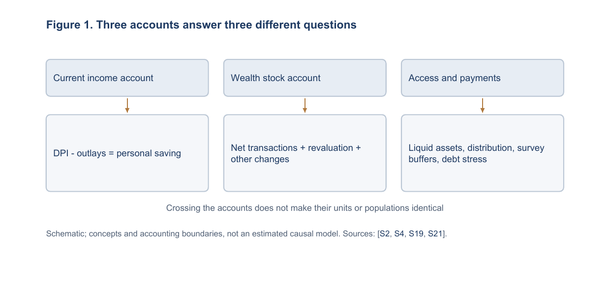
The central research question is whether the post-pandemic saving picture represents a durable weakening of current-income accumulation or a misleading reading of broader balance-sheet strength. Answering it requires keeping three objects separate: the flow left after personal outlays, the stock of accumulated net worth, and assets available for near-term payments. Their units differ, their sector boundaries differ across sources, and their movements need not agree. This article first reconciles each object on its own terms, then crosses them to determine which interpretations survive. [S2, S4, S19]

NIPA personal saving is disposable personal income less personal outlays. Outlays include consumption, personal interest payments and current transfer payments. Disposable income is personal income less personal current taxes. Income includes items such as employer benefit contributions and pension accruals that do not pass through a household’s checking account. Capital gains from asset-price changes are excluded. Saving can finance asset acquisition or debt repayment; it cannot be inferred from deposits alone. The historical series already incorporates the pension methodology adopted in the 2013 comprehensive revision, so that date is not an untreated break in the current observations. [S19, S20, S21]

Net worth changes, by contrast, combine net transactions, revaluation and other changes in volume. The Financial Accounts explicitly report those components. The transactions measure includes accounting for nonfinancial assets and consumer durables and is not interchangeable with NIPA personal saving. A direct wealth reconciliation is stronger than labeling the residual between wealth change and saving as capital gains, because that residual would combine incompatible definitions and adjustments. Financial net lending is another distinct flow: financial-asset acquisition less liabilities incurred. [S4, S5]

These distinctions determine the empirical sequence. The income account identifies the size and arithmetic source of a saving-rate change. The wealth account identifies the origin of stock accumulation. Distributional accounts and surveys test whether aggregate assets describe widespread cash resilience. Forecast models finally ask whether lagged stocks improve prediction beyond the saving rate’s own recent history. A positive finding in one block is not evidence for every other block. This design gives the article falsifiable comparisons rather than a single composite index that hides incompatible concepts.

A common cutoff contains different vintages

The information cutoff is 21 October 2026, but the observations do not share a single release date. The core BEA file was last modified on 30 September and ends in August. Financial Accounts stocks end in 2026Q2 in the 11 September release; the 18 September DFA snapshot uses the same latest quarter but a separate distributional estimation system. The 2025 SCF arrived on 9 October and is therefore inside the cutoff, while the DFA snapshot predates it. Annual SHED evidence refers to adults interviewed in October 2025 and was published in May 2026. [S1, S3, S4, S8, S13]

The primary monthly panel has 188 observations and 16 variables, without missing cells, from January 2011 to August 2026. A separate 2010 seed supports lag construction. Monetary flows are billions of dollars SAAR, real income and consumption use chained 2017 dollars, and population is in thousands. The quarterly balance panel contains the 2010Q4 starting stock plus 62 analysis quarters through 2026Q2. Its original dollar units are millions. The joined model replaces the embedded older NIPA outcomes with current BEA income, outlays and saving while preserving the Fed stock vintage. [S1, S2, S4]

The source architecture is deliberately asymmetric. Monthly macro observations support dense flow accounting; quarterly accounts support exact wealth decomposition; surveys support distribution and financial-resilience comparisons at their actual frequencies. No annual household buffer is invented for an unobserved year, and no monthly debt or wealth value is interpolated to create apparent precision. Complete-quarter aggregation uses exactly three observed months, leaving July to August 2026 outside the quarterly models. [S1, S4, S10, S13]

All reported observations, derived identities and estimates are distinguished in captions. Observed means a released source value, including an official modeled DFA estimate. Identity-derived means arithmetic applied to those observations. Estimated means a fitted regime, coefficient, forecast or statistical interval. The distinction concerns the article’s operation, not a claim that official data are free of measurement error. Retained source snapshots and machine-readable dictionaries make the release timing and units inspectable alongside the estimates.

Source	Snapshot/release	Final observation	Population or unit
BEA monthly	30 Sep 2026	Aug 2026	Personal sector; flows SAAR
Financial Accounts	11 Sep 2026	2026Q2	Households + nonprofits
DFA	18 Sep 2026	2026Q2	Modeled wealth-ranked groups
SCF	9 Oct 2026	Survey 2025	Families; real 2025 dollars
SHED	13 May 2026	Survey 2025	Adults; response percentages
DSR / NY Fed	22 Sep / 11 Aug 2026	2026Q2	Payment ratio / credit panel

Table 2. Release dates and actual coverage. Source: [S1, S4, S6, S9, S16]. Cutoff: 21 October 2026.

The long monthly series resists one trend

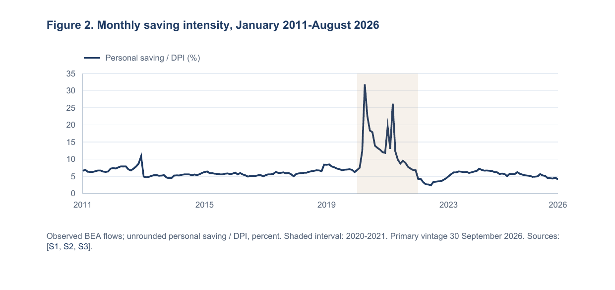
The current monthly saving series is not well described by a monotonic fifteen-year decline. Before the pandemic it moves through distinct episodes: the relatively high 2012 annual result, a lower 2013 to 2016 interval, and a recovery to 7.289% in 2019. The pandemic creates an exceptional upward excursion, followed by the 2022 low and a 2023 to 2024 rebound. The 2025 and observed 2026 values then soften again. Plotting all 188 actual months exposes both the exceptional shock and the shorter movements that a two-endpoint comparison would suppress. [S1]

The figure uses the unrounded ratio 100 times personal saving divided by DPI. This matches the published one-decimal rate after rounding in every month, but avoids injecting one-decimal steps into regressions. At the latest month, the released 4.1% corresponds to $990.229 billion SAAR saving and $24,223.171 billion SAAR DPI. That is an annualized monthly pace, not $990 billion saved during August. The month-equivalent seasonally adjusted flow is the SAAR amount divided by twelve. [S1, S3]

The high pandemic values pose a statistical problem as well as an economic one. A short-lived extreme movement can dominate fitted means, coefficient signs and model selection even when the subsequent normal-period dynamics are the object of interest. It would be equally misleading to erase the event silently. The analysis therefore preserves a full sample and a transparent pandemic-excluded sensitivity, and evaluates forecasting separately inside and outside the event. Quarterly exclusions cover 2020Q1-2021Q4; the supplementary monthly forecast classification follows the explicit dates stored in its output. [S1, S4]

A full-history chart is a diagnostic, not a structural explanation. It demonstrates that a candidate explanation must account for reversals and the scale of the pandemic departure. It cannot establish whether taxes, transfers, inflation, asset prices or preferences caused any local change. The next pages use exact accounting to narrow the arithmetic question and out-of-sample tests to limit behavioral claims. Maintaining that sequence is especially useful when the narrative suggested by a headline month is more confident than the long-run evidence.

Weighted annual rates reveal the rebound

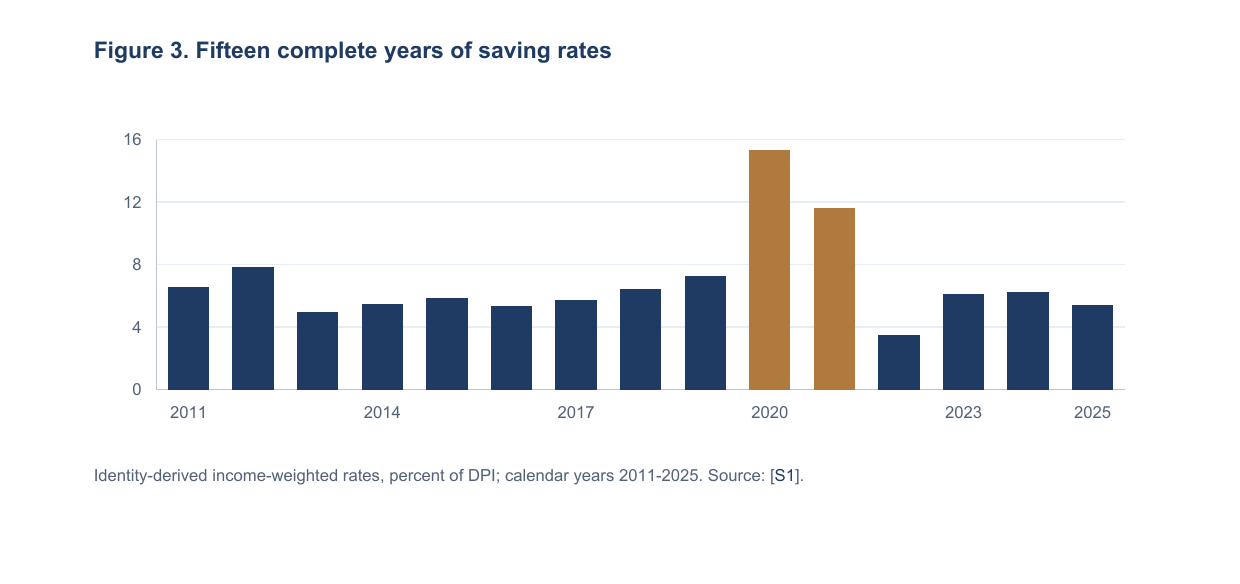
Annual saving intensity must be calculated from annual flows. With monthly seasonally adjusted annual rates S and D, the annual saving rate is 100 times the sum of S divided by the sum of D. This is the DPI-weighted mean of unrounded monthly rates. The annual actual saving flow is the mean of monthly SAAR saving, because each month contributes one-twelfth of its annualized pace. An unweighted average of published rounded rates answers a slightly different question and becomes particularly unreliable when incomes move sharply within a year. [S1, S2]

Using that convention, 2022 is the lowest complete-year rate in this window at 3.485%, while 2020 is the highest at 15.312%. The rebound to 6.116% in 2023 and 6.265% in 2024 matters for the regime claim: a low 2022 does not by itself describe the entire post-2022 interval. The 2025 result of 5.403% is lower again, yet remains above the 2022 trough and the 2013 annual value. The observed pattern is a substantial shock, normalization and further fluctuation rather than a single uninterrupted descent. [S1]

The annual dollar quantity provides a complementary scale. Personal saving in 2025 is $1,241.941 billion against $22,986.000 billion DPI. Dollar saving is affected by growth in prices, population and income, so a higher nominal amount cannot be equated to stronger saving effort. Conversely a rate compares the residual to income and can fall even if the number of dollars saved rises. This is why the article reports both rates and flows, while using real-dollar survey values for comparisons of family balance sheets. [S1, S10]

The 2026 extension is intentionally outside the fifteen-year table. January to August has a 4.737% ratio of observed flows; it is neither the full-year 2026 rate nor a forecast for the remaining months. Its valid recent comparator is January to August 2025, not an unmatched twelve-month total. The same principle governs the quarterly extension: only complete quarters enter stock-flow comparisons. This small accounting discipline prevents coverage differences from becoming economic conclusions.

Year	Rate (%)	Year	Rate (%)	Year	Rate (%)
2011	6.548	2016	5.357	2021	11.635
2012	7.870	2017	5.759	2022	3.485
2013	4.969	2018	6.449	2023	6.116
2014	5.478	2019	7.289	2024	6.265
2015	5.842	2020	15.312	2025	5.403

Table 3. Annual income-weighted saving rates. Source: [S1]; ratios of sums of unrounded monthly flows, 2011 to 2025.

Income growth alone does not preserve saving

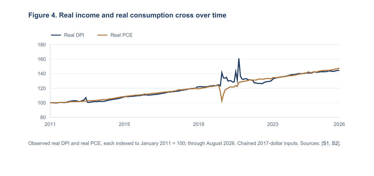
Saving is a relatively small residual between large income and outlay flows. The joint long-run plot therefore matters more than either nominal series on its own. Both DPI and consumption rise substantially across 2011 to 2025, and the recent saving-rate change depends on their relative movement and the nonconsumption outlays that connect PCE to total outlays. A nominal income gain can coincide with lower saving intensity if the share absorbed by spending rises. That statement follows directly from the account and does not require estimating a consumption propensity. [S1, S2]

The figure indexes real DPI and real PCE to their own January 2011 levels. These are two separately observed chained-dollar series, not constructed real saving. The index removes dollar-scale differences and shows when real spending and income follow different paths. It also avoids presenting nominal growth during inflation as a real resource gain. Real DPI minus real PCE omits nonconsumption personal outlays and is therefore not personal saving. Any saving deflated by a stated price index is explicitly a constructed purchasing-power measure. [S1, S2]

The pandemic is visible as a divergence and reversal in flows, while the subsequent period requires matched comparisons. The five-factor decomposition in the full research note works in current dollars and preserves the exact saving identity. It allocates the rate change among nontransfer income, transfers, taxes, PCE and other outlays symmetrically. It is not a decomposition of purchasing power or a claim about households’ preferred consumption. Price changes, quantities and composition all remain inside their observed nominal aggregates. [S1]

This separation is important for interpretation. A spending contribution can be negative in an identity even when households are not voluntarily becoming less cautious; required expenses, demographics, relative prices and income shocks can all influence observed totals. Similarly, transfer income can raise the arithmetic saving rate without a separately identified policy treatment effect. The present data-first exercise establishes the magnitude of the residual and its accounting counterparts. Identifying why those flows changed would require additional variation and a different research design.

Frequently asked questions

Sources

• [S1] BEA monthly National Income and Product Accounts flat file
  30 September 2026 vintage; January 2011 to August 2026 analysis panel. Original nominal flows are converted to billions of dollars SAAR. This is the primary saving outcome source.
• [S2] BEA official series register
  Definitions and codes for personal saving, income, taxes, outlays, consumption, transfers, prices and population. Real flow series use chained 2017 dollars.
• [S3] BEA, Personal Income and Outlays, August 2026
  Released 30 September 2026. Documents the annual update beginning January 2021 and the latest monthly release available at the cutoff.
• [S4] Federal Reserve, Financial Accounts dated data archive
  Released 11 September 2026. S1M balance-sheet, transaction, revaluation and integrated-account files; household and nonprofit stocks through 2026Q2. The embedded NIPA outcome is an older vintage than S1.
• [S5] Federal Reserve, Financial Accounts release
  Dated release and source-table context. The analysis uses direct FC/FU/FR/FV net-worth components, with original amounts in millions of dollars.
• [S6] Federal Reserve, Distributional Financial Accounts data archive
  Snapshot retrieved 21 October 2026, released 18 September 2026. Detailed wealth-ranked group levels and shares; 2011Q1-2026Q2. The retained ZIP fixes this otherwise moving URL.
• [S7] Federal Reserve, DFA methods and visualization
  Scope and construction of group balance sheets. Top 1 percent is included in Top 10 percent; group identities are wealth ranks, not a fixed panel of people.
• [S8] Federal Reserve, DFA announcements
  Explains extrapolation after 2022Q3 and instrument changes. September DFA predates the October 2026 release of the 2025 SCF.
• [S9] Federal Reserve, Survey of Consumer Finances index
  2025 survey released 9 October 2026. Survey design and data documentation; assets at interview and income for the preceding calendar year.
• [S10] Federal Reserve, SCF historical real-dollar tables
  One 2025-dollar vintage for 2010, 2013, 2016, 2019, 2022 and 2025. Table 4 net worth; asset-holder conditional balances and Table 18 debt burden.
• [S11] Federal Reserve, 2025 SCF report
  Definitions of transaction and retirement accounts and debt-payment denominators. Conditional medians and repeated cross-sections are kept distinct from aggregate stocks.
• [S12] Federal Reserve, 2025 SHED savings and investments
  Released 13 May 2026; survey fielded October 2025. Hypothetical $400 payment methods and three-month reserves refer to adults. Footnotes explain threshold experiments.
• [S13] Federal Reserve, SHED chart data archive
  Frozen 13 May 2026 snapshot. Cash-equivalent responses 2013 to 2025 and three-month reserve responses 2015 to 2025; missing earlier reserve cells are preserved.
• [S14] Federal Reserve, debt service ratios
  22 September 2026 snapshot; current-methodology total, mortgage and consumer required-payment ratios through 2026Q2. Retained HTML fixes the release vintage.
• [S15] Federal Reserve, debt service ratio methodology
  Current credit-bureau-based scheduled-payment methodology. The article does not splice legacy debt-service histories to the current series.
• [S16] Federal Reserve Bank of New York, household credit workbook
  Released 11 August 2026. Debt balances and delinquency stocks/flows; 2011Q1-2026Q2 retained panel, workbook pages 3, 12, 13 and 14.
• [S17] New York Fed, Household Debt and Credit technical notes
  Consumer Credit Panel coverage and measurement. Credit-panel balances are distinct from the Financial Accounts household/nonprofit liability total.
• [S18] New York Fed, reconciling credit-card delinquency measures
  11 August 2026 explanation of transitions, four-quarter moving sums and reporting/charge-off effects. Supports careful stock-versus-flow interpretation.
• [S19] BEA, Income and Saving
  Conceptual boundary of current personal income and saving. Capital gains are excluded; some measured income is noncash.
• [S20] BEA, accrual accounting for defined-benefit pension plans
  17 June 2013 methodological explanation. Historical NIPA income and saving incorporate pension accruals, rather than measuring only cash deposited.
• [S21] BEA, Alternative Measures of Personal Saving
  Survey of Current Business, April 2002, conceptual discussion. Used for saving boundaries, not for its superseded pension cash treatment.
• [S22] New York Fed, current household-credit summary
  Q2 2026 summary cautions that mortgage reporting was temporarily affected by a servicing-transfer gap. The workbook, rather than a different-vintage blog number, supplies balances.