A Two-Speed American Economy in 2026: Who Still Benefits from Growth?

A Two-Speed American Economy in 2026: Who Still Benefits from Growth?

Driss EFFINA, PhD Independent Researcher, Global Strategy Files Reading time: about 26 minutes

Abstract

The American economy continued to grow in 2026 despite an oil shock, tariffs and rising interest rates. Real GDP increased at an annual rate of about 2.4 percent in the first half of the year, and the unemployment rate stood at 4.2 percent in September. Yet the Federal Reserve’s Beige Book of 14 October 2026 described an economy in which, in more than half of the twelve Federal Reserve Districts, consumer spending was driven by high-income households, while lower-income households showed growing signs of strain: hardship withdrawals from retirement accounts, more use of buy now, pay later credit, first-time visitors at food pantries and trading down. This article measures the gap between the two speeds of the economy. It combines a systematic coding of the October 2026 Beige Book with official data from the Bureau of Labor Statistics, the Bureau of Economic Analysis and the Federal Reserve Bank of New York, and with the author’s own calculations of inflation by income group. Five results stand out. First, eight of the twelve Districts reported strain on lower- or middle-income households, and seven reported spending led by high-income households. Second, inflation is higher for lower-income households: in September 2026, the CPI for wage earners (CPI-W) rose by 3.9 percent against 3.7 percent for all urban consumers, and the author’s stylised calculation suggests a gap of about 0.4 percentage points between the lowest and highest income quintiles, almost entirely due to energy. Third, real hourly earnings fell by 0.7 percent over the year to September, after rising in 2025. Fourth, credit stress is concentrated in credit card and auto debt, typical of households with fewer assets, while mortgage and home equity delinquency remain low. Fifth, the labour market has not deteriorated broadly, which means that the two-speed pattern is driven by prices and wealth rather than by job losses. The article concludes that the resilience of aggregate demand depends increasingly on wealthy households and on asset prices, which makes the economy more vulnerable to a financial market correction, and that energy relief would benefit lower-income households most.

Keywords: United States, inequality, consumer spending, Beige Book, inflation inequality, household credit, real wages, K-shaped economy, wealth effect

JEL codes: D31, D12, E21, E31, E32

1. Introduction

Aggregate statistics describe the average, and averages can hide very different experiences. In 2026, the American economy offers a striking example. On the one hand, GDP is growing at about its potential rate, unemployment is low by historical standards, corporate investment is booming, and stock prices have been supported by the enthusiasm for artificial intelligence. On the other hand, millions of households are facing higher prices for gasoline, food away from home and insurance, falling real wages, rising borrowing costs and the loss of some public benefits.

The term “two-speed economy”, or “K-shaped economy”, describes a situation in which different groups follow diverging trajectories: one branch of the K goes up, the other goes down. The concept became popular during the recovery from the pandemic, when high-income households benefited from rising asset prices and the ability to work from home, while lower-income households faced job losses in services.

The October 2026 Beige Book, the Federal Reserve’s summary of anecdotal information collected from businesses and community contacts in its twelve Districts, provides a rich description of this divergence. Over half of the Districts reported that consumer spending was driven by high-income households. At the same time, the reports describe many signs of strain among lower- and middle-income households.

This article asks a simple question: who still benefits from growth? It tries to answer it by combining the qualitative evidence of the Beige Book with quantitative evidence on prices, wages, credit and employment, and by calculating how inflation differs across income groups.

Section 2 presents the context. Section 3 reviews the literature. Section 4 describes the data and methods. Section 5 presents the results. Section 6 discusses them. Section 7 presents scenarios. Section 8 concludes.

2. Context

2.1 Aggregate resilience

The American economy has shown remarkable aggregate resilience in 2026. Real GDP grew at an annual rate of 2.5 percent in the first quarter and 2.2 percent in the second quarter, according to the third estimates of the Bureau of Economic Analysis. Real final sales to private domestic purchasers rose by 4.6 percent at an annual rate in the second quarter. The unemployment rate was 4.2 percent in September 2026, lower than a year earlier (4.4 percent).

This resilience has been supported by three forces: a boom in business investment linked to artificial intelligence, examined in a previous article in this series; strong household wealth, driven by stock and housing prices; and a labour market that has remained solid, with low layoffs.

2.2 Shocks that weigh on households

At the same time, households have faced several shocks. The 2026 oil shock pushed the price of regular gasoline to an average of 4.35 dollars per gallon in September, against 3.10 dollars on average in 2025. Consumer price inflation rose to 3.7 percent in September. Tariffs introduced since 2025 raised the price level of goods. Mortgage rates rose to 7.4 percent in October 2026, their highest level since November 2023. And in some states, changes in Medicaid and the Supplemental Nutrition Assistance Program (SNAP) have reduced benefits for some low-income households, as noted by the Boston and New York Districts in the Beige Book.

2.3 The October 2026 Beige Book

The Beige Book of 14 October 2026 reported that economic activity grew in nine of the twelve Districts (two at a moderate pace, three at a modest pace and four slightly) and was unchanged in three. Most Districts reported little or no change in overall consumer spending. Prices rose at a moderate pace in eight Districts and at a robust pace in three, with higher oil prices affecting every District. Employment was broadly flat. Five Districts reported that some firms were reducing staffing through attrition or delayed hiring after investing in AI to raise productivity.

3. Literature review

The analysis draws on four strands of literature.

The first concerns inequality in income and wealth. Piketty and Saez (2003) documented the long-run rise in the share of income going to the top of the distribution in the United States since the 1970s. The Federal Reserve’s Distributional Financial Accounts show that wealth is even more concentrated than income, and that the top tenth of households holds the large majority of directly and indirectly held corporate equities. This concentration means that gains in stock prices benefit mainly high-income households.

The second concerns inflation inequality, the fact that different households face different inflation rates because they consume different baskets. Kaplan and Schulhofer-Wohl (2017), using scanner data, showed that household-level inflation rates vary widely. Jaravel (2021) reviewed the evidence and found that, over long periods, lower-income households have tended to experience higher inflation, partly because of the composition of their spending and partly because innovation and competition have been stronger in products bought by higher-income households. In energy shocks, the difference is amplified, because energy represents a larger share of the budget of lower-income households.

The third concerns the link between household balance sheets and consumption. Mian, Rao and Sufi (2013) showed that the fall in consumption during the Great Recession was concentrated in areas where households had high debt and suffered large falls in housing wealth, and that the marginal propensity to consume out of wealth is higher for poorer households. Poterba (2000) reviewed the evidence on the stock market wealth effect and found that each dollar of stock market wealth raises consumption by a few cents a year. Kaplan, Moll and Violante (2018) showed that, in models with heterogeneous households, monetary policy affects the economy largely through its indirect effects on the incomes of households with few liquid assets.

The fourth concerns the macroeconomic consequences of inequality. Cynamon and Fazzari (2016) argued that the rise in inequality before 2008 was sustained by borrowing by lower-income households, and that the end of this borrowing contributed to the slow recovery after the Great Recession. Chetty and co-authors (2020), using real-time private sector data, showed that the fall in spending at the start of the pandemic came mainly from high-income households, while job losses were concentrated among low-wage workers, an early documentation of the K-shaped pattern.

4. Data and methodology

4.1 Data

The analysis uses:

• the Federal Reserve’s Beige Book of 14 October 2026, national summary and twelve District reports;
• the BLS Consumer Price Index for September 2026, including the CPI-U and the CPI-W;
• the BLS Real Earnings releases for July and September 2026;
• the BLS Employment Situation for September 2026, including unemployment rates by educational attainment and race;
• the BEA Personal Income and Outlays for August 2026;
• the Federal Reserve Bank of New York Household Debt and Credit Report for the second quarter of 2026;
• the Energy Information Administration’s Short-Term Energy Outlook of October 2026.

4.2 Coding the Beige Book

The author read the national summary and the twelve District reports and coded the presence of seven signals: spending driven by high-income households; strain on lower- or middle-income households; price sensitivity or trading down; increased use of buy now, pay later, short-term or hardship credit; fuel prices forcing trade-offs; rising demand at food banks or nonprofits; and weaker consumer credit quality. For the first signal, the national summary states that over half of the Districts reported it; the author therefore codes it at seven, the minimum consistent with this statement. This coding is necessarily subjective, but it provides a systematic summary of the qualitative evidence.

4.3 Inflation by income group

The official CPI-W, which covers households of wage earners and clerical workers, provides a first official comparison with the CPI-U. To go further, the author calculates inflation for five stylised baskets corresponding to income quintiles. The baskets use budget shares that reproduce the main patterns of the BLS Consumer Expenditure Survey: lower-income households spend larger shares on shelter, utilities, food at home, gasoline and health care, and smaller shares on food away from home, vehicles and air travel. The shares are approximations, not official figures. They are combined with the twelve-month inflation rates of the corresponding CPI categories in September 2026: shelter 3.2 percent, electricity and natural gas about 4.6 percent, food at home 1.8 percent, food away from home 3.5 percent, gasoline 34.2 percent, medical care 1.5 percent, apparel 3.4 percent, vehicles about zero (new vehicles +0.6 percent, used vehicles -1.5 percent), airline fares 22.4 percent, and all other items 2.6 percent (the core rate). Because the stylised baskets do not exactly reproduce official weights, the levels of the resulting rates are less reliable than the gap between them.

4.4 Scenarios

The scenarios estimate the effect on annual consumer spending of two shocks that affect households differently: a fall in gasoline prices, which benefits all households but represents a larger share of the budget of lower-income households; and a fall in stock prices, which affects mainly high-income households through the wealth effect. The calculations use an annual gasoline consumption of about 136 billion gallons, household holdings of corporate equities assumed at about 55 trillion dollars, a wealth effect of 3 cents per dollar, and annual consumer spending of about 21 trillion dollars.

4.5 Limitations

The Beige Book is anecdotal and not representative in a statistical sense. The stylised baskets are approximations. The data on unemployment by education are not seasonally adjusted and are volatile month to month. The scenarios are illustrative.

5. Results

5.1 The Beige Book picture

Figure 1 summarises the Beige Book evidence.

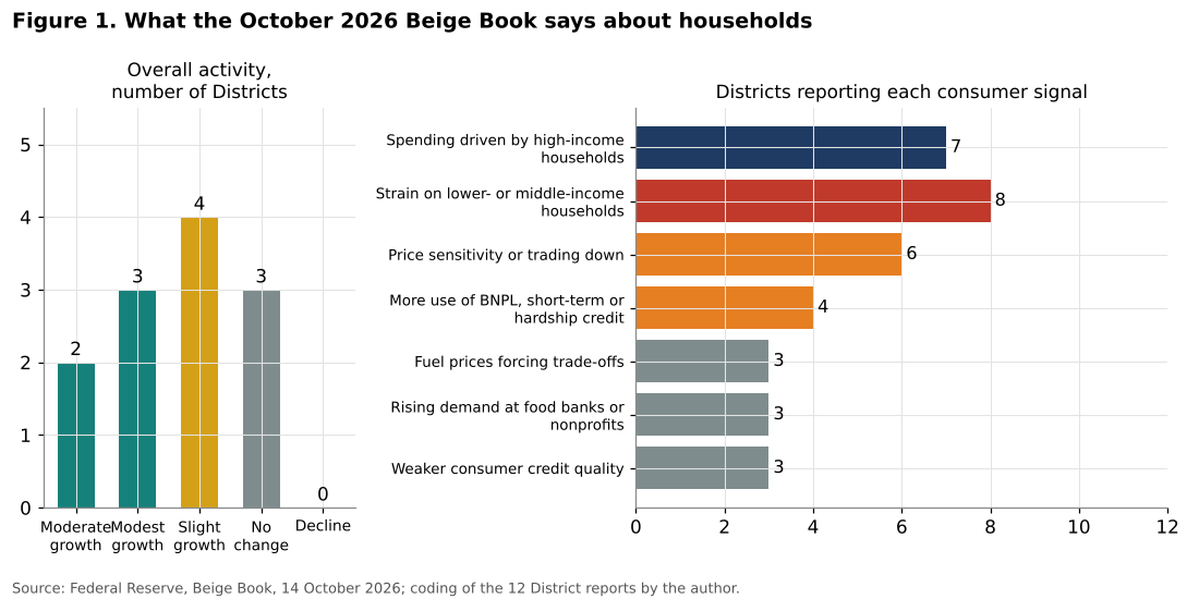
The left panel shows that overall activity was growing in nine Districts and flat in three, with none reporting a decline. The growth was mostly slight to modest. This is an economy that is growing, but slowly.

The right panel shows the frequency of consumer signals. The most frequent signal is strain on lower- or middle-income households, reported in eight Districts: Boston, New York, Cleveland, Atlanta, St. Louis, Minneapolis, Kansas City and Dallas. Spending driven by high-income households was reported in over half of the Districts. Price sensitivity or trading down was reported in six Districts, increased use of buy now, pay later, short-term or hardship credit in four, fuel prices forcing trade-offs in three, rising demand at food banks or nonprofits in three, and weaker consumer credit quality in three.

The District reports provide concrete examples. In New York, lower-income households showed strain through more hardship withdrawals from 401(k) retirement accounts and more use of earned wage advances, and food pantries saw first-time users. In Atlanta, rising fuel and food costs strained low- and moderate-income consumers, while spending on high-end retail offset weakness in other value tiers, and the use of buy now, pay later for groceries and dining grew. In St. Louis, an entertainment venue saw demand shift from high-end to mid-range options, and nonprofits reported middle-income households seeking help with rent and mortgage payments. In Kansas City, households ate at home more, traded down on quality and skipped planned purchases, while small businesses turned to costly merchant cash advances. In Minneapolis, lower-income underemployed workers took second and third jobs. In Cleveland, nonprofits reported a record share of clients whose finances had worsened, and auto customers reduced maintenance to a minimum. In Boston, contacts expected continued strength in higher-end spending but expressed widespread concern about cost pressures on lower-income families.

These anecdotes describe a coherent pattern. Higher-income households continue to spend, supporting aggregate consumption and high-end businesses. Lower- and middle-income households are adjusting: trading down, postponing purchases, using more expensive forms of credit and, in some cases, seeking assistance.

5.2 Inflation is not the same for everyone

Figure 2 shows the author’s estimates of inflation by income quintile in September 2026.

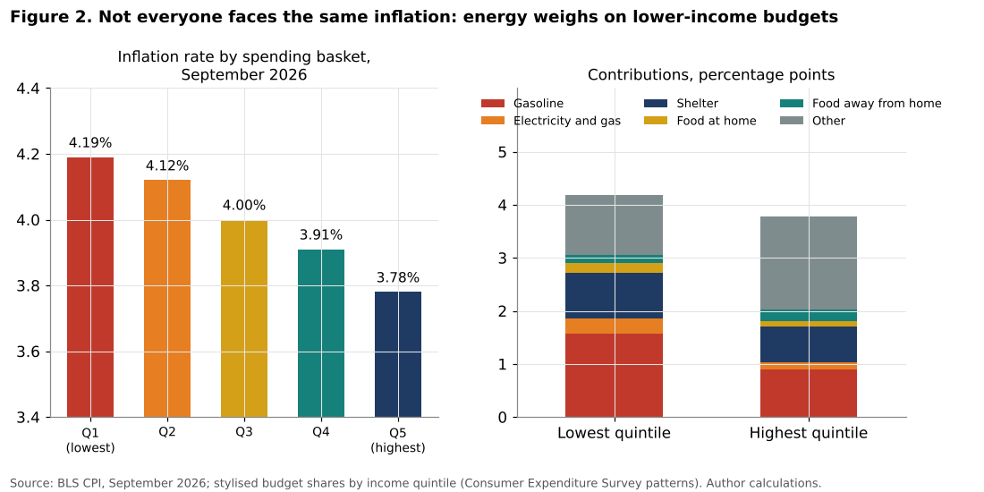
According to these estimates, inflation was about 4.2 percent for the stylised basket of the lowest quintile, against about 3.8 percent for the highest quintile, a gap of about 0.4 percentage points. The gap is almost entirely due to energy. Gasoline and household energy (electricity and natural gas) contributed about 1.85 percentage points to the inflation of the lowest quintile, against about 1.03 points for the highest quintile. The highest quintile spends more on airline fares, which rose by 22.4 percent, and on food away from home, which rose by 3.5 percent, but these categories carry less weight than gasoline.

The official data confirm this pattern. The CPI-W, which covers households of wage earners, whose incomes are on average lower than those of all urban consumers, rose by 3.9 percent over the year to September 2026, against 3.7 percent for the CPI-U. In July 2026, before the September energy spike, both indexes had risen by 3.3 percent. The divergence of September is therefore directly linked to the energy shock.

The difference may seem small, but it is significant for household budgets. For a household with annual spending of 40,000 dollars, an additional 0.4 percentage points of inflation represents 160 dollars a year, on top of the general increase in prices. And the gasoline shock itself is large: each one dollar increase in the price of a gallon of gasoline costs American households about 136 billion dollars a year in total, or about 1,030 dollars per household on average. Between 2025 (average price 3.10 dollars) and 2026 (expected average 3.91 dollars), the national gasoline bill increased by about 110 billion dollars.

5.3 Real wages

Figure 3 shows inflation and real wages.

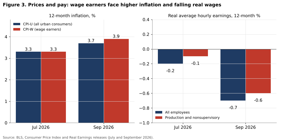
Real average hourly earnings, which measure the purchasing power of wages, fell by 0.7 percent over the year to September 2026 for all employees, and by 0.6 percent for production and nonsupervisory employees. In July, the declines were only 0.2 and 0.1 percent. Nominal hourly earnings rose by 3.0 percent for all employees and 3.3 percent for production and nonsupervisory employees, but not enough to keep up with prices.

The fact that the decline in real wages is similar for both groups, despite the higher inflation faced by wage earners, reflects the slightly faster nominal wage growth of production and nonsupervisory employees. However, this measure covers only workers who are employed. It does not capture the situation of people who are not working, retirees on fixed incomes, or recipients of public benefits that have been reduced.

At the aggregate level, real disposable personal income was unchanged in August 2026, and the personal saving rate was 4.1 percent. A low saving rate means that, on average, households are maintaining their consumption by saving less. But averages are misleading here: high-income households may be reducing their saving out of choice, because their wealth has increased, while lower-income households may be doing so out of necessity, because their real incomes are falling.

5.4 Credit stress

Figure 4 shows the flow into serious delinquency by type of debt.

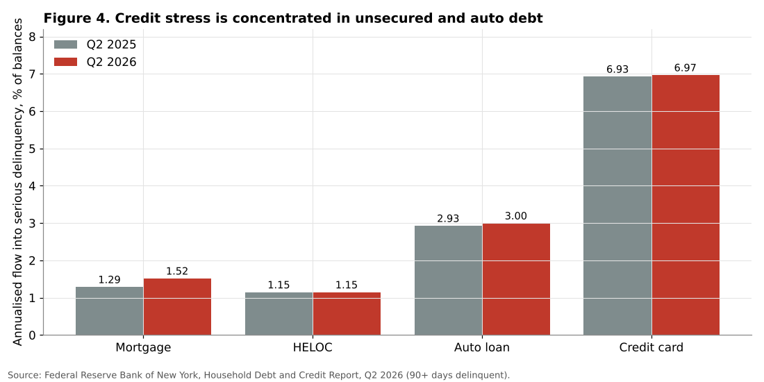
The data of the Federal Reserve Bank of New York for the second quarter of 2026 show that the annualised flow of credit card balances into serious delinquency (90 days or more) was 6.97 percent, against 6.93 percent a year earlier. For auto loans, it was 3.00 percent, against 2.93 percent. These are elevated levels, as the New York Fed noted. For mortgages, the flow rose from 1.29 to 1.52 percent, still low by historical standards, and for home equity lines of credit it was unchanged at 1.15 percent.

The contrast between types of debt is informative. Mortgages and home equity lines are held mainly by homeowners, who are on average wealthier and have benefited from rising house prices. Many of them also locked in low fixed rates before 2022. Credit card and auto debt, by contrast, are used more by households with fewer assets, for whom these forms of credit are a way to bridge gaps in income. Credit card balances reached 1.263 trillion dollars in the second quarter of 2026, 54 billion dollars more than a year earlier.

The Beige Book adds qualitative detail: consumer creditworthiness declined in Atlanta, consumer loan quality deteriorated slightly in Chicago, and past-due loans were slightly elevated in Richmond. The use of buy now, pay later credit for everyday purchases such as groceries and dining, reported in Atlanta and St. Louis, is a particular warning sign, because it indicates that some households are using credit to finance basic consumption.

5.5 The labour market: no broad deterioration

Figure 5 shows unemployment rates by educational attainment.

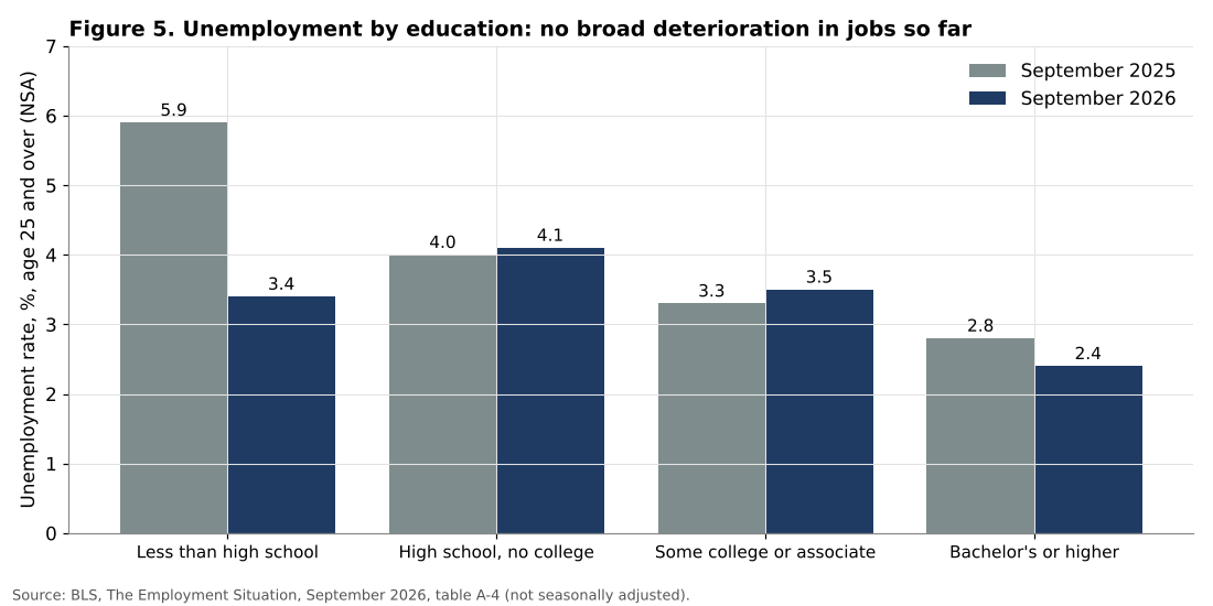
One of the most important findings is that the two-speed pattern of 2026 is not, for now, driven by unemployment. Unemployment rates by educational attainment (not seasonally adjusted, for people aged 25 and over) did not show a broad deterioration between September 2025 and September 2026: the rate for high school graduates without college was 4.1 percent against 4.0 percent, the rate for those with some college was 3.5 percent against 3.3 percent, and the rate for college graduates fell from 2.8 to 2.4 percent. The rate for those without a high school diploma fell from 5.9 to 3.4 percent, a decline that should be interpreted with caution given the volatility of this series. Unemployment rates also fell for Black workers (from 7.3 to 6.8 percent), Hispanic workers (from 5.3 to 4.5 percent) and Asian workers (from 4.4 to 2.9 percent).

This is an important difference from previous downturns, in which lower-income households suffered mainly from job losses. In 2026, they suffer mainly from prices: energy, food away from home, insurance, and the cost of credit. This distinction matters for policy, because the appropriate responses differ.

There are, however, signs of future risks in the labour market. Payroll growth has been weak, with a gain of only 29,000 jobs in September and a decline of 10,000 in July after revision. Five Beige Book Districts reported firms reducing staffing through attrition or delayed hiring after investing in AI. Governor Lisa Cook noted in September that recent college graduates face more difficulty finding first jobs. If the labour market weakens, the two-speed pattern could become more severe.

5.6 Wealth: the hidden driver

The other branch of the K is driven by wealth. Stock prices have been supported in 2025 and 2026 by the enthusiasm for artificial intelligence, and house prices remain high. Since corporate equities are heavily concentrated among the wealthiest households, rising stock prices increase their wealth and support their spending through the wealth effect. The Beige Book observation that spending is driven by high-income households in over half of the Districts is consistent with this mechanism.

This creates an unusual situation. In a typical expansion, consumption is supported by rising employment and wages across the distribution. In 2026, aggregate consumption is supported to a significant extent by the spending of high-income households, which depends on asset prices. The economy is therefore more dependent on financial markets than usual, and more vulnerable to a correction.

5.7 A second dimension: regions and sectors

The two speeds of the economy are not only a matter of income. The Beige Book also shows marked differences between regions and sectors. Dallas reported robust, broad-based growth in manufacturing, and six other Districts reported modest to moderate manufacturing growth, while services outside manufacturing showed little overall growth. Richmond reported moderate growth, solid consumer spending despite trade-offs linked to gasoline prices, and strong hotel occupancy. By contrast, Chicago, Kansas City and San Francisco reported flat activity. In Kansas City, rising diesel prices and shipping costs squeezed profit margins, and in Chicago, farm income expectations for 2026 were revised slightly down.

Some regional differences reflect specific shocks. Boston, Minneapolis and San Francisco reported lower sales to Canadian tourists, a consequence of the trade tensions between the United States and Canada. Boston reported a sharp rise in home heating oil prices from a year earlier, which matters for households in the Northeast as winter approaches. Atlanta reported moderate growth in energy activity, which benefits from higher oil prices, illustrating that the energy shock creates winners as well as losers inside the United States.

These regional contrasts reinforce the income contrast. Regions specialised in energy production, advanced manufacturing or data centre construction benefit from the current configuration of the economy. Regions that depend on agriculture, on consumer services for middle-income households, or on cross-border tourism with Canada face more difficult conditions. Within each region, the households most exposed to fuel and food prices bear the heaviest burden.

6. Discussion

6.1 Who benefits from growth?

The evidence presented in this article allows a clear answer to the question asked in the title. In 2026, the main beneficiaries of growth are households with significant financial and housing wealth, who have benefited from rising asset prices and, in many cases, from fixed-rate mortgages contracted at low rates, and workers in sectors linked to the AI investment boom, such as construction of data centres and electrical work. Businesses serving high-income customers, such as high-end retail, travel and hospitality, are also doing well.

The households that benefit least are those with low or moderate incomes and few assets, who spend a large share of their budget on energy, food and transport, who rent rather than own, who rely on credit cards and auto loans, and who may have lost some public benefits. For these households, the 2026 economy is one of falling real wages, rising prices and rising borrowing costs.

6.2 Why it matters for the macroeconomy

The two-speed pattern is not only a question of fairness. It has macroeconomic consequences.

First, it makes aggregate demand more fragile. If consumption depends on the spending of wealthy households, which depends on asset prices, a stock market correction could produce a sharp slowdown in consumption, even if the labour market remains solid.

Second, it complicates monetary policy. Higher interest rates reduce inflation partly by reducing the spending of households that depend on credit, who are disproportionately lower-income. But they may have less effect on wealthy households, whose spending depends on wealth and who may even benefit from higher returns on savings. A monetary tightening may therefore increase the burden on the more vulnerable households without significantly slowing the spending of the wealthiest.

Third, it may affect political attitudes and policy choices. A large gap between aggregate statistics and the experience of many households can undermine confidence in institutions and in economic policy, and increase support for measures such as tariffs or price controls that may have significant costs.

6.3 Energy as the key variable

The analysis shows that energy is the main source of the difference in inflation between income groups in 2026. This has an encouraging implication: if energy prices fall in 2027, as forecast by the Energy Information Administration, lower-income households will benefit more than proportionally. The fall in gasoline prices forecast by the EIA, from 4.35 dollars in September 2026 to about 3.56 dollars on average in 2027, would reduce the gap in inflation between income groups and support the real incomes of the most constrained households.

6.4 The role of credit

The rising use of buy now, pay later and other short-term credit to finance everyday purchases is a warning sign. These forms of credit are convenient but can lead to over-indebtedness, especially for households with irregular incomes. They are also less well captured by traditional credit statistics. The stability of delinquency rates on credit cards at elevated levels suggests that the situation is not yet deteriorating rapidly, but the combination of falling real wages and rising interest rates creates a risk of a gradual increase in defaults, as the New York Fed has noted for auto loans and credit cards.

6.5 Policy options

Several policy options could reduce the gap between the two speeds of the economy, each with its own trade-offs. Targeted support for lower-income households facing energy costs, such as energy assistance programmes, would be more efficient than broad measures, but requires fiscal resources. Reducing tariffs on goods consumed by lower-income households would lower their cost of living but reduce revenue and protection. Monetary policy could look through energy shocks to avoid adding a recession to an energy shock, but this risks the credibility of the inflation target. These are choices that involve value judgements and that this article does not attempt to settle.

6.6 Lessons from earlier episodes

The K-shaped pattern is not new. After the global financial crisis, the recovery of asset prices, supported by very low interest rates and quantitative easing, benefited mainly wealthy households, while the recovery of employment and wages for lower-income workers took nearly a decade. During the pandemic, high-income households saved massively while low-wage workers lost their jobs, before the very tight labour market of 2021 and 2022 produced the fastest wage growth at the bottom of the distribution in decades.

The 2026 episode differs from both. Unlike 2009, there is no mass unemployment. Unlike 2021, wages at the bottom are not rising faster than prices. The squeeze comes from prices, and in particular from energy, a pattern closer to the oil shocks of the 1970s than to recent cycles. The lesson from the 1970s is that the distributional effects of energy shocks can be long-lasting if they feed into persistent inflation, which is one reason why the Federal Reserve is watching inflation expectations closely, as discussed in an earlier article in this series.

7. Scenarios

7.1 Two shocks, two speeds

Figure 6 shows the estimated effect on annual consumer spending of three scenarios.

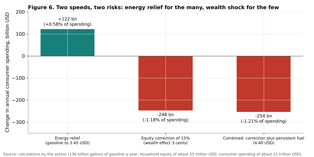
Energy relief. If gasoline prices fall from 4.35 dollars per gallon in September 2026 to about 3.45 dollars, as implied by the EIA forecasts for late 2027, households would save about 122 billion dollars a year on fuel, equivalent to about 0.58 percent of consumer spending. This relief would benefit all households, but represent a larger share of the budget of lower-income households.

Equity correction. If stock prices fall by 15 percent, household equity wealth would fall by about 8 trillion dollars, assuming household holdings of about 55 trillion dollars. With a wealth effect of 3 cents per dollar, consumer spending would fall by about 248 billion dollars a year, or about 1.18 percent. This effect would be concentrated among high-income households.

Combined stress. If an equity correction coincided with persistent high fuel prices (4.40 dollars per gallon), consumer spending would fall by about 254 billion dollars, or 1.21 percent. In this scenario, both branches of the K would be under pressure at the same time: the wealthy because of the fall in their wealth, the others because of high energy prices.

7.2 Interpretation

The scenarios show that the risks facing the American consumer in 2027 are asymmetric. The main upside, energy relief, would mostly benefit lower-income households and would support consumption modestly. The main downside, an equity correction, would mostly affect high-income households, but its effect on aggregate consumption would be about twice as large, because these households account for a large share of total spending.

This reflects the paradox of the two-speed economy: the spending of the wealthiest has become the main support of aggregate demand, so that the economy is most vulnerable to shocks that affect them, even though the households under the most strain are elsewhere.

7.3 Indicators to monitor

The author suggests monitoring:

1. the gap between the CPI-W and the CPI-U, as an indicator of inflation inequality; 2. real average hourly earnings for production and nonsupervisory employees; 3. flows into delinquency on credit cards and auto loans, and the use of buy now, pay later credit; 4. the Beige Book descriptions of spending by income group; 5. stock prices and their effect on the wealth of high-income households.

8. Conclusion

This article has examined the two-speed American economy in 2026. The main conclusions are:

1. The October 2026 Beige Book describes an economy in which spending is driven by high-income households in over half of the Districts, while eight Districts report strain on lower- or middle-income households. 2. Inflation is higher for lower-income households, mainly because of energy: the CPI-W rose by 3.9 percent in September 2026 against 3.7 percent for the CPI-U, and the author’s stylised estimates show a gap of about 0.4 percentage points between the lowest and highest income quintiles. 3. Real hourly earnings fell by 0.7 percent over the year to September 2026. 4. Credit stress is concentrated in credit card and auto debt, while mortgage and home equity delinquency remain low. 5. The labour market has not deteriorated broadly, so the two-speed pattern is driven by prices and wealth rather than by unemployment.

Who still benefits from growth? Mainly households with significant wealth and those linked to the investment boom. The others are not losing their jobs, but they are losing purchasing power and resorting more to credit. The resilience of aggregate demand depends increasingly on wealthy households and on asset prices, which makes the economy more vulnerable to a financial correction. A fall in energy prices in 2027 would bring relief to the most constrained households, but the structural gap between the two speeds of the economy, rooted in the distribution of wealth, is likely to persist.

Frequently asked questions

Methodological note

The Beige Book coding was carried out by the author on the basis of the national summary and the twelve District reports published on 14 October 2026. The inflation estimates by income quintile use stylised budget shares that reproduce the main patterns of the BLS Consumer Expenditure Survey, combined with September 2026 CPI category inflation rates; they are approximations intended to illustrate the gap between groups. Other data are taken from official releases of the BLS, BEA, Federal Reserve Bank of New York and EIA. The scenarios rely on stated assumptions and are illustrative.

References

Board of Governors of the Federal Reserve System (2026). The Beige Book: Summary of Commentary on Current Economic Conditions by Federal Reserve District. 14 October 2026.

Board of Governors of the Federal Reserve System (2026). Distributional Financial Accounts. Washington, DC.

Bureau of Labor Statistics (2026). Consumer Price Index, September 2026; Real Earnings, July and September 2026; The Employment Situation, September 2026. Washington, DC.

Chetty, R., Friedman, J. N., Hendren, N., Stepner, M. and the Opportunity Insights Team (2020). The Economic Impacts of COVID-19: Evidence from a New Public Database Built Using Private Sector Data. NBER Working Paper 27431.

Cynamon, B. Z. and Fazzari, S. M. (2016). Inequality, the Great Recession and Slow Recovery. Cambridge Journal of Economics, 40(2), 373 to 399.

Energy Information Administration (2026). Short-Term Energy Outlook, October 2026. Washington, DC.

Federal Reserve Bank of New York (2026). Household Debt and Credit Report, Q2 2026. 11 August 2026.

Jaravel, X. (2021). Inflation Inequality: Measurement, Causes, and Policy Implications. Annual Review of Economics, 13, 599 to 629.

Kaplan, G., Moll, B. and Violante, G. L. (2018). Monetary Policy According to HANK. American Economic Review, 108(3), 697 to 743.

Kaplan, G. and Schulhofer-Wohl, S. (2017). Inflation at the Household Level. Journal of Monetary Economics, 91, 19 to 38.

Mian, A., Rao, K. and Sufi, A. (2013). Household Balance Sheets, Consumption, and the Economic Slump. Quarterly Journal of Economics, 128(4), 1687 to 1726.

Piketty, T. and Saez, E. (2003). Income Inequality in the United States, 1913 to 1998. Quarterly Journal of Economics, 118(1), 1 to 41.

Poterba, J. M. (2000). Stock Market Wealth and Consumption. Journal of Economic Perspectives, 14(2), 99 to 118.