The Return of Inflationary Pressure in the United States: How Far Should the Federal Reserve Go?

The Return of Inflationary Pressure in the United States: How Far Should the Federal Reserve Go?

Driss EFFINA, PhD Independent Researcher, Global Strategy Files Reading time: about 27 minutes

Abstract

In September 2026, consumer prices in the United States rose by 0.6 percent in a single month and by 3.7 percent over twelve months, the highest annual rate since 2023. A week before the release, on 16 September, the Federal Open Market Committee had raised the federal funds target range by a quarter point to 3.75 to 4.00 percent, its first increase since July 2023. This article examines the nature of the new inflationary episode and the appropriate scale of the monetary response. Using the September 2026 Consumer Price Index of the Bureau of Labor Statistics, the August 2026 personal income and outlays release of the Bureau of Economic Analysis, the Federal Reserve’s September Summary of Economic Projections, the Short-Term Energy Outlook of the Energy Information Administration and household credit data from the Federal Reserve Bank of New York, the author computes the contribution of each component to headline inflation, the recent momentum of core prices, the real policy rate under several definitions, a set of Taylor rule prescriptions and three oil price scenarios to the end of 2027. Five results stand out. First, energy accounts for about 1.45 percentage points of the 3.7 percent headline rate, and gasoline alone for about 1.27 points; consumer prices excluding energy rose by only about 2.4 percent. Second, core inflation remains moderate on a twelve-month basis (2.6 percent for the CPI, 3.0 percent for the PCE), but its three-month annualised pace accelerated to 3.4 percent in September. Third, real average hourly earnings fell by 0.7 percent over the year, the clearest sign that the energy shock is eroding purchasing power. Fourth, financing conditions have tightened well beyond the policy rate: the 30-year mortgage rate reached 7.4 percent in October, against 6.27 percent a year earlier, and long-term Treasury yields are close to their highest levels since 2007. Fifth, simple policy rules place the appropriate federal funds rate between 4.25 and 5.30 percent, above the current midpoint of 3.875 percent. The article concludes that the Fed faces a classic supply shock dilemma in which the main risk is not the direct effect of energy prices, which should fade in 2027, but their transmission to core prices and expectations. A measured response, with one further increase and a long pause, appears more consistent with the evidence than either a return to easing or an aggressive tightening cycle.

Keywords: United States, inflation, Federal Reserve, oil price shock, energy prices, monetary policy, Taylor rule, real wages, credit conditions

JEL codes: E31, E43, E52, E58, Q43

1. Introduction

For most of 2025 and the first months of 2026, the debate about American monetary policy was about how fast the Federal Reserve should cut interest rates. After reducing the federal funds rate by 100 basis points in late 2024 and by a further 75 basis points between September and December 2025, the Fed held its target range at 3.50 to 3.75 percent and waited for inflation to settle near its 2 percent objective. In January and February 2026, headline consumer price inflation was 2.4 percent, among the lowest rates since 2021, and the remaining question seemed to be whether one or two more cuts would be needed.

The escalation of the conflict in the Middle East changed the picture. Oil supply through the Strait of Hormuz was severely disrupted from the spring of 2026. According to the Energy Information Administration, crude oil shut-ins in the region peaked at 10.9 million barrels per day in May. Brent crude, which had averaged 63.63 dollars per barrel in the fourth quarter of 2025, averaged 102.93 dollars in the second quarter of 2026 and 114 dollars in September, with a daily high of 131 dollars on 15 September after attacks on the Saudi East-West pipeline, the main route bypassing the Strait. American gasoline prices followed: regular gasoline averaged 4.35 dollars per gallon in September 2026, and diesel 6.29 dollars.

Consumer price inflation rose to 3.3 percent in March, 4.2 percent in May, eased to around 3.4 percent in the summer as oil prices fell back temporarily, and rose again to 3.7 percent in September. On 16 September, the Federal Open Market Committee (FOMC) voted unanimously to raise the target range to 3.75 to 4.00 percent, “in support of the Federal Reserve’s dual mandate”. The September Summary of Economic Projections showed a median federal funds rate of 4.1 percent at the end of 2026, implying one more increase before the end of the year.

This raises the question that the Fed has faced in every oil shock since the 1970s: should monetary policy respond to a rise in prices that originates in a supply disruption abroad and that, in principle, will reverse when the disruption ends? Or should it treat the shock as a threat to the anchoring of inflation expectations, and tighten even at the cost of slower growth?

This article answers this question with the evidence available in mid-October 2026. Section 2 sets out the context. Section 3 reviews the literature on oil shocks and monetary policy. Section 4 describes the data and methods. Section 5 presents the results. Section 6 discusses them. Section 7 presents scenarios to the end of 2027. Section 8 concludes.

2. Context

2.1 The disinflation of 2023 to 2025

After peaking at 9.1 percent in June 2022, the highest rate in four decades, consumer price inflation fell rapidly in 2023 as energy prices declined, supply chains normalised and the Fed raised its policy rate to 5.25 to 5.50 percent. By June 2023, inflation was down to 3.0 percent. The last mile proved more difficult: headline inflation fluctuated between 2.3 and 3.5 percent through 2024 and 2025, while core inflation, which excludes food and energy, declined slowly from about 4 percent at the start of 2024 to about 3 percent in 2025.

The Fed began to cut rates in September 2024 and brought the target range down to 4.25 to 4.50 percent by December 2024. It then paused for most of 2025, partly because of uncertainty about the inflationary effect of tariffs, before cutting three more times between September and December 2025. In October and November 2025, a lapse in federal appropriations interrupted the publication of some statistics, and the CPI for October 2025 was never published.

2.2 The 2026 energy shock

The 2026 oil shock is the third major energy shock of the century for the American economy, after the price surge of 2007 to 2008 and the rise that followed the invasion of Ukraine in 2022. Its distinctive features are its origin in a physical disruption of shipping routes rather than in demand, and its duration. According to the EIA, shut-ins were still 4.8 million barrels per day in September 2026 and are expected to average 4.5 million barrels per day in the fourth quarter, with most production returning to pre-conflict levels only by the end of the second quarter of 2027.

The United States is now a net exporter of petroleum, which changes the macroeconomic effect of an oil shock compared with the 1970s. Higher oil prices raise the income of American producers and the value of exports, which partly offsets the loss of purchasing power of consumers. But the distribution of the effect is uneven: consumers in all regions pay more at the pump, while the gains are concentrated in producing states and among shareholders of energy companies.

2.3 The September 2026 CPI

The September 2026 CPI, published on 14 October, showed the following:

Category	Monthly change (SA)	12-month change
All items	+0.6%	+3.7%
Energy	+5.2%	+20.4%
Gasoline	+9.1%	+34.2%
Fuel oil	+15.3%	+74.2%
Electricity	+0.2%	+4.4%
Food	0.0%	+2.5%
Core (all items less food and energy)	+0.3%	+2.6%
Shelter	+0.4%	+3.2%
Services less energy services	+0.4%	+3.1%
Core goods	+0.3%	+0.7%
Airline fares	+1.2%	+22.4%

Table 1. Consumer Price Index, September 2026. Source: BLS.

The BLS noted that gasoline accounted for more than half of the monthly increase in the headline index. Core inflation was 0.3 percent for the second consecutive month, slightly above market expectations. Airline fares, which depend on jet fuel costs, rose by 22.4 percent over the year, an early sign of the transmission of energy costs to services.

2.4 The Fed’s September decision

The FOMC statement of 16 September described economic activity as expanding at a solid pace, with resilient domestic spending, strong productivity growth and robust capital investment. Job gains had kept pace with the growth of the workforce and the unemployment rate had changed little. Inflation remained elevated. The increase in the policy rate was intended to support “a timelier return” to the 2 percent goal.

On 29 September, the President of the Federal Reserve Bank of New York, John Williams, explained that he now expected “somewhat larger and longer-lasting effects from energy prices on inflation”, but that he had not seen evidence of broader and persistent inflation spreading from current pressures. He suggested that, if the economy evolved as he expected, one further increase in the target range might be appropriate late in the year. He also noted that tariffs were no longer adding to goods price inflation, and that demand linked to investment in artificial intelligence was becoming an increasingly salient source of price pressure.

3. Literature review

The literature on oil shocks and monetary policy is large. Four contributions are especially relevant.

The first concerns the macroeconomic effects of oil shocks. Hamilton (1983) showed that almost every American recession after the Second World War had been preceded by a sharp increase in oil prices, establishing oil shocks as a central macroeconomic variable. Kilian (2009) refined this view by showing that “not all oil price shocks are alike”: shocks driven by supply disruptions, by global demand or by precautionary demand have very different effects on prices and output. The 2026 episode is clearly a supply disruption, combined with a rise in precautionary demand linked to the risk of further disruption.

The second concerns the role of monetary policy. Bernanke, Gertler and Watson (1997) argued that a large part of the output losses that followed oil shocks in the 1970s and 1980s was due not to the shocks themselves but to the monetary tightening that followed them. This conclusion has been debated, but it remains a warning against an excessive response to supply shocks. Blanchard and Galí (2007) showed that the effects of oil shocks on inflation and output became much smaller after the mid-1980s, and attributed this to three factors: a smaller share of oil in the economy, more flexible labour markets and, above all, the improved credibility of monetary policy, which kept inflation expectations anchored.

The third concerns expectations. Coibion and Gorodnichenko (2015) showed that household inflation expectations are strongly influenced by gasoline prices, which households observe frequently. This creates a channel through which an energy shock can affect wage demands and price setting even if it is temporary. Kilian and Zhou (2022) estimated the effect of the 2020 to 2022 oil price increase on American inflation and on household expectations, and found that the effect on expectations was significant but that the effect on core inflation was modest.

The fourth concerns the post-pandemic inflation episode. Bernanke and Blanchard (2023) decomposed the inflation of 2021 to 2023 and showed that it began as a series of price shocks, especially in energy and food, but that its persistence depended on labour market tightness. Their framework is useful for 2026: the initial shock is clearly energy, and the question is whether labour market conditions and expectations will turn it into persistent inflation.

Finally, the literature on monetary policy rules, initiated by Taylor (1993), provides a benchmark for assessing the level of the policy rate. These rules are not meant to be applied mechanically, but they summarise the response that has historically been associated with good macroeconomic outcomes.

4. Data and methodology

4.1 Data

The main sources are:

• the BLS Consumer Price Index news release for September 2026 (14 October 2026), including relative importance weights for December 2025;
• the history of the CPI-U twelve-month change (not seasonally adjusted) and the seasonally adjusted core CPI index from 2018 to September 2026;
• the BLS Real Earnings release for September 2026 and earlier releases;
• the BLS Employment Situation for September 2026;
• the BEA Personal Income and Outlays release for August 2026;
• the FOMC statement and Summary of Economic Projections of 16 September 2026;
• the EIA Short-Term Energy Outlook of October 2026;
• the Federal Reserve Bank of New York Household Debt and Credit Report for the second quarter of 2026;
• Freddie Mac weekly mortgage rates.

4.2 Contributions to inflation

The contribution of a component to twelve-month inflation is approximated by its relative importance weight multiplied by its twelve-month change. The December 2025 weights are: energy 7.418 percent (of which gasoline 3.853), core goods 18.835 percent, core services 60.240 percent, and food the remainder, 13.507 percent. Because weights drift with relative prices during the year, the raw contributions sum to slightly more than the headline rate (3.91 points against 3.7 percent). The author scales them proportionally so that they sum to the published headline rate. Consumer price inflation excluding energy is then estimated as the headline rate minus the energy contribution, divided by the non-energy weight.

4.3 Core momentum

Three-month and six-month annualised rates of change of the seasonally adjusted core CPI index are calculated as ((index in month t / index in month t-k) to the power 12/k, minus 1). For periods that include October 2025, for which no index was published, the calculation uses the actual number of months between available observations.

4.4 Real interest rates and policy rules

The real federal funds rate is calculated as the midpoint of the target range (3.875 percent) minus three measures of inflation: headline CPI, core CPI and core PCE. The policy rule is the original Taylor (1993) rule:

Rule rate = r + π + 0.5 × (π – 2) + 0.5 × output gap*

The output gap is approximated by Okun’s law as minus twice the gap between the unemployment rate (4.2 percent in September 2026) and its longer-run level (4.2 percent in the FOMC median projection), which gives a gap of zero. Two measures of inflation are used, core PCE (3.0 percent) and headline PCE (3.4 percent) for August 2026, and two values of the neutral real rate: 0.75 percent, close to many model estimates, and 1.2 percent, which corresponds to the FOMC median longer-run nominal rate of 3.2 percent minus the 2 percent target.

4.5 Oil scenarios

The scenarios project headline CPI inflation at the end of 2027 using a simple decomposition: headline inflation equals the weighted sum of core inflation (weight 79.1 percent), food inflation (13.5 percent, assumed at 2.5 percent) and energy inflation (7.4 percent). Energy inflation is assumed to move by 0.8 times the percentage change in gasoline prices, reflecting the weight of gasoline within energy and the slower movement of electricity and gas tariffs. Gasoline prices at the end of 2027 are derived from the assumed Brent price using the rule of thumb that 10 dollars per barrel corresponds to about 24 cents per gallon (one barrel contains 42 gallons).

4.6 Limitations

The contributions are approximations. The policy rules ignore the uncertainty about the neutral rate and the output gap. The scenarios are illustrative and ignore second-round effects beyond the assumed core inflation path. Real wage data for some months are taken from BLS summaries rather than from a complete series.

5. Results

5.1 Inflation and the policy rate in perspective

Figure 1 shows headline and core CPI inflation together with the upper bound of the federal funds target range since 2019.

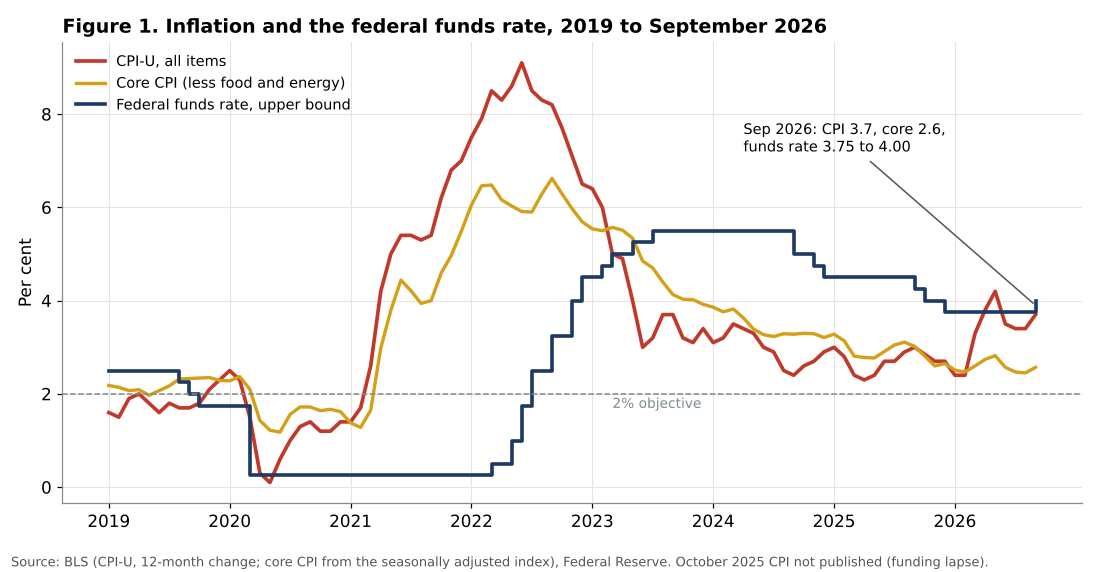
The chart shows three episodes. In 2021 and 2022, inflation surged while the policy rate remained near zero until March 2022, a delay that the Fed itself later acknowledged. From 2023, the policy rate was well above inflation, and inflation declined. In 2025, the policy rate was cut while core inflation was still around 3 percent.

The 2026 episode looks different from 2021 and 2022 in one crucial respect: core inflation has not followed headline inflation upward. In September 2026, headline inflation was 3.7 percent while core inflation was 2.6 percent, a gap of more than one percentage point. In 2021, both rose together. This suggests that, so far, the shock is concentrated in energy and has not spread broadly to other prices.

5.2 What makes up 3.7 percent inflation

Figure 2 shows the contribution of each major component to twelve-month inflation in September 2026.

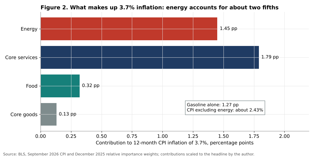
According to the author’s calculations, energy contributed about 1.45 percentage points to the 3.7 percent headline rate, core services about 1.79 points, food about 0.32 points and core goods about 0.13 points. Gasoline alone contributed about 1.27 points, more than a third of headline inflation, even though it represents less than 4 percent of the consumer basket.

Consumer price inflation excluding energy was therefore about 2.4 percent, close to the 2 percent objective once the usual difference between the CPI and the PCE index is taken into account. Without the energy shock, the United States would have an inflation rate broadly consistent with the Fed’s target.

Two caveats are necessary. First, core services inflation (3.1 percent) remains above the rate compatible with the target, mainly because of shelter (3.2 percent), whose decline has been slow. Second, the core PCE index, which the Fed uses as its preferred measure, rose by 3.0 percent over the twelve months to August 2026, more than the core CPI. The two indexes differ in their weights and coverage, and the PCE measure currently points to more persistent underlying inflation than the CPI.

5.3 Monthly swings and core momentum

Figure 3 shows the monthly changes in headline, core and energy prices in 2026 and the momentum of core inflation.

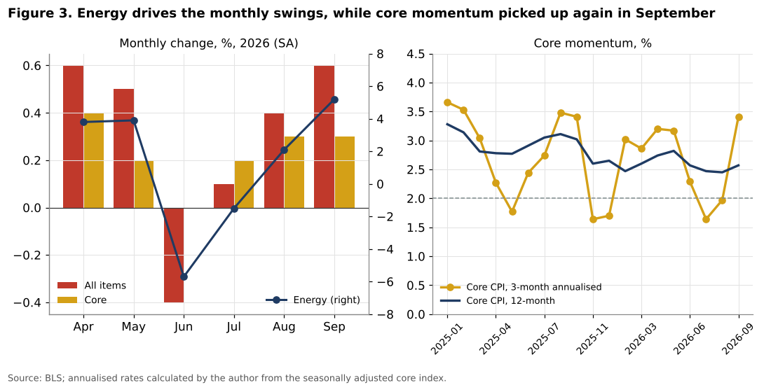
The left panel shows that the monthly path of headline inflation is driven by energy. Energy prices rose by 3.8 and 3.9 percent in April and May, fell by 5.7 percent in June as oil prices temporarily declined, then rose again by 2.1 percent in August and 5.2 percent in September. Headline inflation followed: +0.6 percent in April, -0.4 percent in June, +0.6 percent in September.

The right panel shows the three-month annualised rate of core inflation, a measure of recent momentum. It is volatile, but its recent movement is a warning. After falling to 1.6 percent in July and 2.0 percent in August, it rose to 3.4 percent in September. The six-month annualised rate was 2.9 percent. Over twelve months, core inflation rose from 2.4 percent in August to 2.6 percent in September.

The details of the September release show signs of transmission from energy to other prices. Airline fares rose by 1.2 percent in the month and 22.4 percent over the year. Transportation services rose by 0.6 percent. Motor vehicle maintenance and repair rose by 5.8 percent over the year. These are the categories through which energy costs typically enter core inflation.

5.4 The oil shock

Figure 4 shows the quarterly average price of Brent crude oil from 2025 to 2027, including EIA forecasts, and the retail price of regular gasoline in 2026.

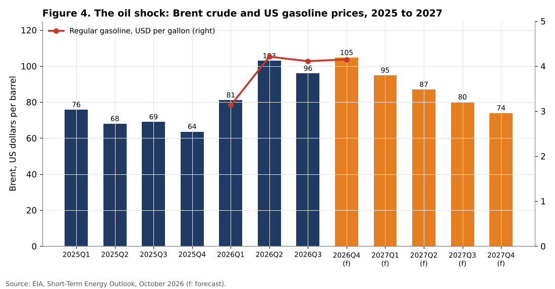
The scale of the shock is clear. Brent averaged 69 dollars per barrel in 2025 and is expected by the EIA to average 96 dollars in 2026, an increase of 40 percent. The fourth quarter of 2026 is expected to be the most expensive, at about 105 dollars. The EIA then expects a gradual decline in 2027, to about 74 dollars in the fourth quarter, as production in the Gulf resumes.

Gasoline prices rose from 3.13 dollars per gallon in the first quarter of 2026 to 4.21 dollars in the second quarter, 4.11 dollars in the third quarter and an expected 4.15 dollars in the fourth quarter. The EIA forecasts an average of 3.56 dollars in 2027. Diesel prices, which affect freight transport and therefore the prices of many goods, are expected to remain above 4 dollars per gallon through 2027 because distillate inventories remain low.

A simple calculation helps measure the sensitivity of inflation to oil prices. Each 10 dollar per barrel change in the price of crude oil changes the price of gasoline by about 24 cents per gallon. At the September price of 4.35 dollars, this represents about 5.5 percent of the price, and, with a weight of 3.85 percent, about 0.21 percentage points of headline CPI inflation. The difference between Brent at 69 dollars (the 2025 average) and at 114 dollars (the September 2026 average) therefore represents roughly 0.9 to 1.0 percentage points of headline inflation through gasoline alone, before taking into account diesel, heating oil, jet fuel and indirect effects.

5.5 Purchasing power and credit

Figure 5 shows two channels through which the shock affects households: real wages and the cost of credit.

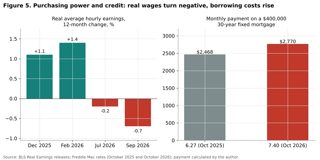
Real average hourly earnings, which had risen by 1.1 percent over the year to December 2025 and by 1.4 percent over the year to February 2026, fell by 0.2 percent over the year to July 2026 and by 0.7 percent over the year to September 2026. Nominal average hourly earnings rose by 3.0 percent over the year to September, less than the 3.7 percent rise in consumer prices. For production and nonsupervisory employees, real hourly earnings fell by 0.6 percent. Real disposable personal income was unchanged in August, and the personal saving rate was 4.1 percent, a low level that leaves households with little buffer.

The labour market provides little compensation. The unemployment rate was 4.2 percent in September 2026, lower than a year earlier (4.4 percent), but payroll employment grew by only 29,000 in September, and the July figure was revised to a decline of 10,000. Labour force participation, at 61.8 percent, was lower than a year earlier.

Credit conditions have tightened considerably, and much more than the 25 basis point increase in the policy rate would suggest. The 30-year fixed mortgage rate measured by Freddie Mac was 7.40 percent on 15 October 2026, its highest level since November 2023, against 6.27 percent a year earlier. On a 400,000 dollar loan, this difference raises the monthly payment from about 2,468 dollars to about 2,770 dollars, an increase of about 301 dollars per month, or more than 3,600 dollars per year. The 10-year Treasury yield approached 5.2 percent in late September, near its highest level since 2007, and the 30-year yield was about 5.48 percent.

Household balance sheets show signs of strain. According to the Federal Reserve Bank of New York, total household debt was 18.77 trillion dollars in the second quarter of 2026. Credit card balances were 1.263 trillion dollars, 54 billion more than a year earlier. The annualised rate of transition of credit card balances into serious delinquency was 6.97 percent, and for auto loans 3.00 percent, levels described by the New York Fed as elevated. The rate for mortgages rose from 1.29 to 1.52 percent over the year. These figures predate the September increase in energy prices and the rise in mortgage rates.

5.6 How restrictive is monetary policy?

The real federal funds rate depends on the measure of inflation used. Measured against headline CPI inflation (3.7 percent), it is only about 0.2 percent, which would suggest that policy is barely restrictive. Measured against core CPI inflation (2.6 percent), it is about 1.3 percent. Measured against core PCE inflation (3.0 percent), it is about 0.9 percent.

The choice of measure is not neutral. If the Fed looks through the energy shock, as standard theory recommends for temporary supply shocks, the relevant measure is core inflation, and policy is moderately restrictive. If it fears that the shock will become persistent, the relevant measure is closer to headline inflation, and policy is close to neutral.

Moreover, financial conditions have tightened independently of the policy rate. The rise in long-term yields, driven according to market commentary by inflation concerns and expectations of further tightening, raises borrowing costs for households and firms. In this sense, part of the tightening that the Fed might otherwise have to engineer through its policy rate is already being done by the bond market.

5.7 What do policy rules say?

Figure 6, left panel, shows the prescriptions of the Taylor (1993) rule under four combinations of assumptions.

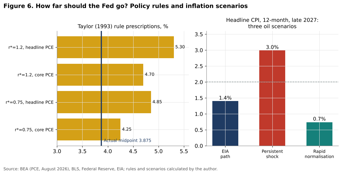
With a neutral real rate of 0.75 percent and core PCE inflation, the rule prescribes 4.25 percent. With a neutral real rate of 1.2 percent and core PCE inflation, it prescribes 4.70 percent. With headline PCE inflation, the prescriptions are 4.85 and 5.30 percent. All four are above the current midpoint of 3.875 percent, by between 0.4 and 1.4 percentage points.

The rules therefore support the September increase and suggest that there is room for at least one more. The FOMC median projection of 4.1 percent at the end of 2026 is at the lower end of the range of rule prescriptions, which is consistent with the Fed’s stated intention to look partly through the energy shock. A policy rate above 5 percent would only be justified if the Fed responded fully to headline inflation, which would amount to treating the energy shock as permanent.

6. Discussion

6.1 A supply shock, not (yet) an inflationary spiral

The central result of this analysis is that the 2026 inflationary episode is, so far, mainly an energy shock. Energy accounts for about two fifths of headline inflation, and inflation excluding energy is close to the target. Core inflation over twelve months is moderate. This is very different from 2021 and 2022, when inflation spread rapidly to all categories of goods and services, driven by strong demand and very tight labour markets.

According to the standard prescription of monetary theory, a central bank should look through the direct effects of a temporary supply shock, because tightening policy cannot increase the supply of oil and would only add a fall in demand to the fall in supply. This was the lesson drawn by Bernanke, Gertler and Watson (1997) from the experience of the 1970s.

But the same literature also shows that this prescription has limits. A central bank can only look through a supply shock if inflation expectations remain anchored. When households see gasoline prices rise every week, their inflation expectations rise too, as Coibion and Gorodnichenko (2015) have shown. And after five years in which inflation has been above target, the credibility of the 2 percent objective is less solid than it was in 2019. This is the main justification for the September increase: it is less a response to current inflation than a signal intended to prevent expectations from drifting.

6.2 Signs of transmission

The September data contain the first signs of transmission from energy to core prices. The acceleration of core momentum, the rise in airline fares and transportation services, and the persistence of shelter inflation are all warning signals. The core PCE index, at 3.0 percent, is also more worrying than the core CPI.

At the same time, other indicators point in the opposite direction. Wage growth has slowed to 3.0 percent, which is roughly consistent with 2 percent inflation given productivity growth that the FOMC describes as strong. Real wages are falling, which reduces the risk of a wage-price spiral. Core goods inflation is low, at 0.7 percent, and the effect of tariffs on goods prices appears to have run its course, according to President Williams.

6.3 The cost of a strong response

A strong monetary response would have significant costs. The economy is already slowing: payroll growth is weak, real disposable income is stagnating and the saving rate is low. Household credit indicators show strain, especially for credit cards and auto loans, which are used disproportionately by lower-income households. The rise in mortgage rates is weighing on the housing market. And the oil shock itself acts as a tax on consumers, reducing their spending on other goods and services.

An aggressive tightening, for example to above 5 percent, would add to these pressures at a time when the shock is expected to fade in 2027. There is a real risk, highlighted by the historical literature, that the combination of an oil shock and a monetary tightening could push the economy into recession, as in 1974, 1980 and 1990.

6.4 The cost of inaction

Conversely, a return to easing, or an extended pause at the current level, would also have costs. Inflation has been above 2 percent for more than five years. If households and firms come to believe that the Fed will tolerate 3 to 4 percent inflation whenever there is a supply shock, expectations could become unanchored, and the cost of bringing inflation back to target would be much higher later. The rise in long-term yields to their highest levels since 2007 may partly reflect a rise in the inflation risk premium demanded by investors, which would be a sign of eroding credibility.

6.5 The distributional dimension

The energy shock and the monetary response affect households unequally. Lower-income households spend a larger share of their budget on gasoline and energy, and they rely more on credit cards and auto loans, whose costs are rising. Higher-income households are more likely to own their homes with fixed-rate mortgages contracted at low rates, and to benefit from higher returns on savings. The fall in real wages, the rise in delinquencies and the low saving rate suggest that the burden of the 2026 shock falls disproportionately on the more vulnerable households. This theme is developed in a later article in this series on the two-speed American economy.

6.6 The fiscal and global context

The rise in long-term yields also reflects factors beyond inflation, including the size of federal deficits and the global rise in yields. Many central banks have begun to tighten in response to the same energy shock, which raises interest rates globally. This global dimension limits the Fed’s ability to influence long-term rates and means that financial conditions could tighten further even if the Fed stops raising its policy rate.

7. Scenarios to the end of 2027

7.1 Three oil price paths

Figure 6, right panel, shows twelve-month headline CPI inflation at the end of 2027 under three oil price scenarios.

Scenario 1: EIA path. Brent declines gradually to about 74 dollars per barrel in the fourth quarter of 2027, in line with the October 2026 Short-Term Energy Outlook. Gasoline falls to about 3.45 dollars per gallon. Core CPI inflation stabilises at about 2.6 percent. Headline inflation falls to about 1.4 percent at the end of 2027, as energy prices decline by more than 10 percent over the year. In this scenario, the energy shock reverses and pulls headline inflation below core inflation. The Fed could hold the rate at around 4 percent through mid-2027 and then begin to ease, consistent with the FOMC median projection of 3.9 percent for 2028.

Scenario 2: Persistent shock. The disruption lasts longer, and Brent stays around 110 dollars. Gasoline rises to about 4.40 dollars. Second-round effects raise core inflation to about 2.9 percent. Headline inflation is about 3.0 percent at the end of 2027, a third consecutive year above target. In this scenario, the Fed would probably need to raise rates to between 4.5 and 5 percent and keep them there, with a significant risk of recession.

Scenario 3: Rapid normalisation. A rapid resolution of the conflict brings Brent back to about 65 dollars, its 2025 level. Gasoline falls to about 3.10 dollars. Core inflation eases to 2.4 percent. Headline inflation falls to about 0.7 percent at the end of 2027 because of the sharp fall in energy prices. In this scenario, the September increase would be reversed relatively quickly.

7.2 Assessment

The scenarios show the asymmetry of the Fed’s problem. In two of the three scenarios, headline inflation falls well below 2 percent in 2027 because of the reversal of energy prices. Only in the persistent shock scenario does inflation remain significantly above target. This argues for caution: if the shock reverses as expected, a policy rate tightened too much in late 2026 would become excessively restrictive in 2027.

However, the uncertainty about the duration of the shock is high, and the cost of being wrong on the side of too little tightening, in terms of credibility, is also high. On balance, the author considers that the evidence supports one further increase of 25 basis points, as signalled by the FOMC median projection and by President Williams, followed by a long pause. This would bring the policy rate to around 4.1 percent, at the lower end of the range of rule prescriptions, which is appropriate for a central bank that looks partly through a supply shock.

7.3 Indicators to monitor

The author suggests monitoring:

1. the three-month annualised rate of core CPI and core PCE inflation, especially services excluding shelter; 2. household inflation expectations, which are sensitive to gasoline prices; 3. long-term Treasury yields and the inflation risk premium; 4. the price of Brent and the volume of shut-ins in the Gulf; 5. delinquency rates on credit cards and auto loans, as indicators of stress among lower-income households.

8. Conclusion

This article has examined the return of inflationary pressure in the United States in 2026. The main conclusions are:

1. The rise of headline inflation to 3.7 percent in September 2026 is mainly due to energy, which contributes about 1.45 percentage points. Inflation excluding energy is about 2.4 percent. 2. Core inflation is moderate on a twelve-month basis (2.6 percent for the CPI, 3.0 percent for the PCE), but its recent momentum has accelerated, and there are first signs of transmission from energy to services. 3. The shock is eroding purchasing power: real hourly earnings fell by 0.7 percent over the year, and credit conditions have tightened sharply, with mortgage rates at 7.4 percent and long-term yields near their highest levels since 2007. 4. Simple policy rules place the appropriate policy rate between 4.25 and 5.30 percent, above the current midpoint of 3.875 percent. 5. In most plausible oil price scenarios, headline inflation falls well below 2 percent in 2027 as energy prices decline.

How far should the Fed go? The evidence suggests a measured answer: far enough to protect the anchoring of inflation expectations, but not so far as to add a monetary contraction to an energy shock that is expected to fade. One more increase followed by a long pause is the path most consistent with the data available in October 2026. The September 2026 CPI showed that the risks are not only on one side, and the coming months, especially the evolution of core services prices and household expectations, will determine whether this measured approach is sufficient.

Frequently asked questions

Methodological note

All calculations were carried out by the author using official data. CPI data come from the BLS release of 14 October 2026 and the historical CPI-U series; the core CPI index is the seasonally adjusted series (FRED code CPILFESL). Contributions are calculated with December 2025 relative importance weights and scaled to the published headline rate. Real interest rates use the midpoint of the target range. The Taylor rule uses the original 1993 coefficients. The oil scenarios use a simplified decomposition of the CPI and should be read as illustrations rather than forecasts. Mortgage payments are calculated with the standard annuity formula for a 30-year fixed-rate loan. Nothing in this article constitutes investment advice.

References

Bernanke, B. S. and Blanchard, O. (2023). What Caused the US Pandemic-Era Inflation? NBER Working Paper 31417.

Bernanke, B. S., Gertler, M. and Watson, M. (1997). Systematic Monetary Policy and the Effects of Oil Price Shocks. Brookings Papers on Economic Activity, 1997(1), 91 to 157.

Blanchard, O. J. and Galí, J. (2007). The Macroeconomic Effects of Oil Price Shocks: Why Are the 2000s So Different from the 1970s? NBER Working Paper 13368.

Bureau of Economic Analysis (2026). Personal Income and Outlays, August 2026. News release, 30 September 2026.

Bureau of Labor Statistics (2026). Consumer Price Index, September 2026. News release USDL-26-1574, 14 October 2026.

Bureau of Labor Statistics (2026). Real Earnings, September 2026. News release, 14 October 2026.

Bureau of Labor Statistics (2026). The Employment Situation, September 2026. News release, 2 October 2026.

Coibion, O. and Gorodnichenko, Y. (2015). Is the Phillips Curve Alive and Well after All? Inflation Expectations and the Missing Disinflation. American Economic Journal: Macroeconomics, 7(1), 197 to 232.

Energy Information Administration (2026). Short-Term Energy Outlook, October 2026. Washington, DC.

Federal Open Market Committee (2026). Federal Reserve Issues FOMC Statement. Press release, 16 September 2026.

Federal Open Market Committee (2026). Summary of Economic Projections, 16 September 2026.

Federal Reserve Bank of New York (2026). Household Debt and Credit Report, Q2 2026. 11 August 2026.

Federal Reserve Bank of New York (2026). Key Takeaways from President Williams’ Speech on the Economic Outlook and Monetary Policy. The Teller Window, 29 September 2026.

Hamilton, J. D. (1983). Oil and the Macroeconomy since World War II. Journal of Political Economy, 91(2), 228 to 248.

Kilian, L. (2009). Not All Oil Price Shocks Are Alike: Disentangling Demand and Supply Shocks in the Crude Oil Market. American Economic Review, 99(3), 1053 to 1069.

Kilian, L. and Zhou, X. (2022). The Impact of Rising Oil Prices on U.S. Inflation and Inflation Expectations in 2020 to 23. Energy Economics, 113, 106228.

Taylor, J. B. (1993). Discretion versus Policy Rules in Practice. Carnegie-Rochester Conference Series on Public Policy, 39, 195 to 214.