
The Herd Arithmetic: Why America’s Record Beef Prices Will Outlast the Political Remedies

Driss EFFINA, PhD Independent Researcher, Global Strategy Files. Decoded, 11 November 2026. Reading time: about 12 minutes.
Key takeaways
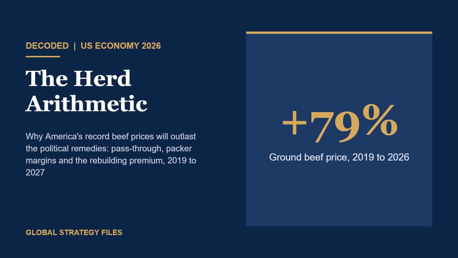
- A pound of ground beef cost $6.80 on average in 2026, 79% more than in 2019. Over the same period consumer prices rose 30% and hourly pay 34%. An American worker now needs 10.9 minutes of work to buy one pound, against 8.2 minutes in 2019 and 6.6 minutes in 2006.
- Ground beef now costs 3.44 times as much as a pound of whole chicken (August 2026), the widest gap in more than thirty years of BLS data. In January 2000 the ratio was 1.40.
- The scarcity rent sits upstream. Between 2019 and 2026, slaughter cattle prices rose 121%, meat packers’ output prices 60% and retail ground beef 79%. The data describe a packer squeeze, not a packer windfall.
- Our distributed-lag model on 321 months of data shows that retail beef absorbs almost nothing of a cattle price change in the same month, about half within six months, and a long-run share of 0.42 to 0.45. Price declines travel at least as fast as increases.
- Cattle prices fell 15.1% between May and September 2026. Retail prices have not yet moved. The model implies an underlying decline of about 8.6% before trend inflation, which puts ground beef near $6.55 to $6.65 in early 2027.
- The cure raises prices before it lowers them. Holding back heifers to rebuild the herd by 5% would cut beef output by about 3% and add roughly 4% to prices in 2027 and 2028. Lasting relief arrives from 2029. The Argentine quota increase equals only 0.5% of US output.
A price that votes
Few prices are as visible to American households as the price of ground beef. It is bought weekly, it sits at the centre of the family budget for protein, and it has become a political number. Over the past year Washington has tried three remedies. In October 2025 the administration announced that it would quadruple the low-tariff quota for Argentine beef from 20,000 to 80,000 metric tons. In November 2025 the President asked the Department of Justice to investigate the four large meatpackers for collusion and price manipulation, and the Attorney General said the investigation was already under way. In 2026 the Department of Agriculture began reopening the southern border to Mexican feeder cattle, closed since 2025 to stop the New World screwworm: the port of Douglas, Arizona, reopened on 24 August and Columbus, New Mexico, on 26 October.
Each remedy rests on a theory of why beef is expensive. The import theory says supply is short and can be topped up from abroad. The antitrust theory says that processors are capturing an excessive margin. The border theory says that a specific policy shock removed a large flow of animals. These theories are not equally supported by the data, and they imply very different timetables for relief.
This article tests them with public data from the Bureau of Labor Statistics, the Department of Agriculture and the Federal Reserve’s FRED database. We measure how expensive beef has become in terms that households understand, decompose the price increase along the supply chain, estimate how fast and how fully cattle prices reach the meat counter, and build an explicit supply ledger for the herd rebuilding phase. Our central conclusion is simple. Beef prices are governed by the biology of the cattle cycle, and that cycle runs on a timetable of years, not of electoral seasons.
How expensive is beef, really?
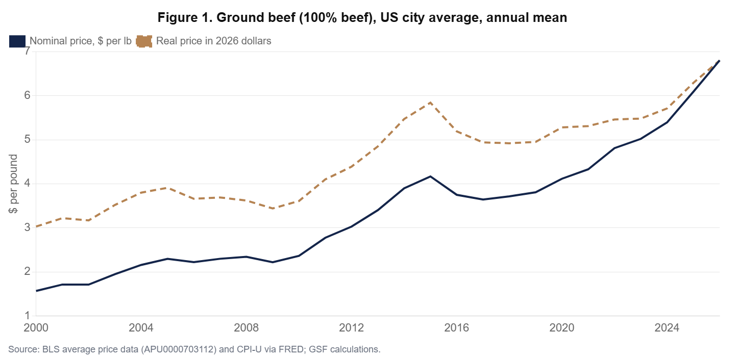
The nominal series tells the first story. The average retail price of 100% ground beef rose from $1.57 per pound in 2000 to $3.81 in 2019 and $6.80 in the first ten months of 2026. Nominal prices, however, overstate the burden in an economy where everything else also costs more. Deflating by the consumer price index, the real price of ground beef in 2026 dollars was $3.03 in 2000, $4.95 in 2019 and $6.80 today. The real increase since 2019 is 37%. The previous real peak, in 2015, was $5.84, which means that today’s price is 16% above the top of the last cattle cycle even after correcting for general inflation (Figure 1).
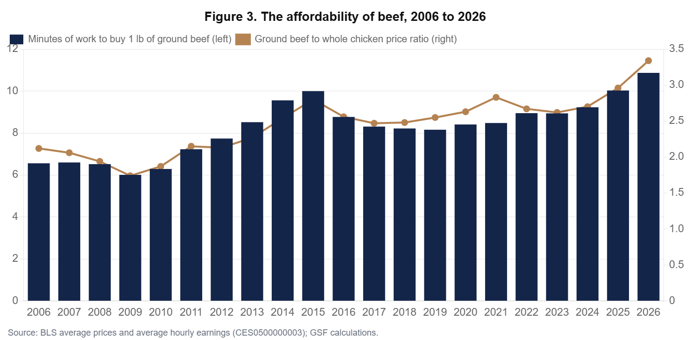
A second way to measure the burden is in working time. Dividing the price per pound by average hourly earnings of private employees gives the minutes of work needed to buy one pound. The measure was 6.6 minutes in 2006, rose to 10.0 minutes at the 2015 peak, fell back to 8.2 minutes in 2019 and has now reached 10.9 minutes, a new high in the twenty-year history of the earnings series. In other words, the wage gains of the past seven years, which were real for most workers, have not kept pace with beef.
The third measure is relative to substitutes. Households respond to expensive beef by buying more chicken, and the ratio of the two prices shows how strong that incentive has become. In January 2000 a pound of ground beef cost 1.40 times a pound of whole chicken. The ratio was 2.66 in December 2019. In August 2026 it reached 3.44, the highest value in our sample since 1995. Chicken prices have barely moved since 2024, while beef has kept climbing (Figure 3).
Despite this, American demand for beef has held up remarkably well. US beef consumption in 2026 is about 8% above its twenty-year average according to the Federal Reserve Bank of Kansas City, while domestic production remains below its historical norm. The gap has been filled by imports, which rose by about 48% in volume between 2020 and 2025 according to the American Farm Bureau Federation. A product whose price has risen 79% in seven years and whose consumption remains above average is not a product suffering from a demand collapse. It is a product facing a supply wall.
Table 1. Price changes along the beef chain and in the wider economy, 2019 to 2026
| Series (annual average) | 2019 | 2026 | Change |
|---|---|---|---|
| Slaughter cattle, PPI (index) | 171.1 | 378.2 | +121% |
| Meat packing output prices, PPI (index) | 186.1 | 296.9 | +60% |
| Retail ground beef ($ per lb) | 3.81 | 6.80 | +79% |
| Retail sirloin steak ($ per lb) | 8.37 | 14.25 | +70% |
| Retail whole chicken ($ per lb) | 1.50 | 2.03 | +36% |
| Retail pork chops ($ per lb) | 3.34 | 4.25 | +27% |
| CPI, food at home (index) | 241.8 | 320.4 | +33% |
| CPI, all items (index) | 255.7 | 332.4 | +30% |
| Average hourly earnings, private ($) | 28.00 | 37.55 | +34% |
The supply wall in numbers
The Department of Agriculture counted 86.2 million cattle and calves on US farms and ranches on 1 January 2026, the smallest inventory since 1951 and about 8.5 million head below the last cyclical peak in 2019. The beef cow herd, the factory of future beef, stood at 27.6 million head, its lowest level since 1961. The 2025 calf crop, at 32.9 million head, was the smallest since 1941, and the July 2026 report expects a 2026 crop of 32.5 million, a further 2% decline.
Three forces produced this contraction. The first is drought, which burned pastures across the Plains between 2020 and 2023 and forced ranchers to sell breeding cows. The second is cost: feed, labour, land and interest rates all rose sharply, which lowered the expected return on keeping a heifer for breeding rather than selling her for slaughter. The third is the border. Mexico supplied an average of 1.17 million feeder cattle a year between 2004 and 2023. The screwworm closure reduced that flow to almost nothing for most of 2025 and the first half of 2026, and agricultural economists at Oklahoma State University expect only 150,000 to 250,000 head to cross in what remains of 2026.
The signs of rebuilding are faint. Beef replacement heifers on 1 January 2026 numbered 4.71 million, up only 1% on the year. That is 17% of the beef cow herd, compared with an average retention rate of about 21%, or 6.2 million head, during the aggressive rebuilding of 2015 to 2018. The herd is not yet growing. It has stopped shrinking quickly.
Who captures the scarcity?
The antitrust theory of high beef prices deserves a careful test, because the four largest packers do control the large majority of US fed cattle slaughter and three of them have paid settlements in past price-fixing litigation without admitting wrongdoing. The question for 2026 is narrower: did processor margins widen enough to explain the price increase since 2019?
Figure 2 answers with three indices set at 100 in 2019. The red line is the producer price index for slaughter cattle, which measures what packers pay ranchers and feeders. The grey line is the producer price index for the output of the meat slaughtering industry. The blue line is the retail price of ground beef. Until 2022 the three lines moved together, with two short episodes of wide packer margins: the pandemic plant closures of spring 2020 and the demand surge of 2021. From 2023 onward the picture changes completely. Cattle prices doubled; packer output prices rose far less.
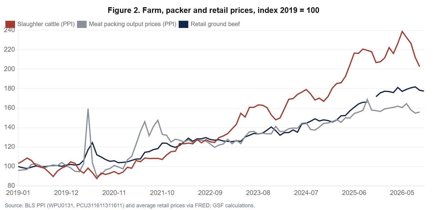
On annual averages, slaughter cattle prices rose 121% between 2019 and 2026 while packer output prices rose 60% (Table 1). Because cattle account for the bulk of a packer’s costs, a gap of this size is incompatible with a widening processing margin. It points to the opposite. The packer index includes pork, which has been cheap, and this overstates the squeeze somewhat; but the direction is unambiguous and matches what the packers themselves report: their trade association said in November 2025 that beef packers had been losing money for more than a year. Retail ground beef, at +79%, sits between the two, which suggests that retailers and the lean imported trim blended into ground beef have absorbed part of the cattle shock.
Our reading is that the 2023 to 2026 surge is a scarcity rent that accrues upstream, to cow-calf operators and feeders who own the scarce animals. That is how a competitive market is supposed to signal a shortage: high prices for calves and heifers are the incentive to rebuild. An investigation may well uncover misconduct, and competition enforcement has its own justification. But it cannot be expected to lower beef prices materially, because the margin it would compress has already been compressed by the market.
Measuring pass-through: how fast does the farm reach the fork?
To quantify the link between cattle and retail prices, we estimate a distributed-lag model on monthly data from January 2000 to September 2026. The dependent variable is the monthly log change in the retail price of ground beef. The explanatory variables are the log change in the slaughter cattle producer price index in the same month and in each of the six previous months, plus the previous month’s retail change to capture adjustment dynamics. The sample has 314 usable observations after lags and two months with missing retail data.
Table 2. Distributed-lag model of retail ground beef prices on slaughter cattle prices
| Term | Coefficient | Std. error | Cumulative |
|---|---|---|---|
| Constant (monthly drift) | 0.0033 | 0.0014 | |
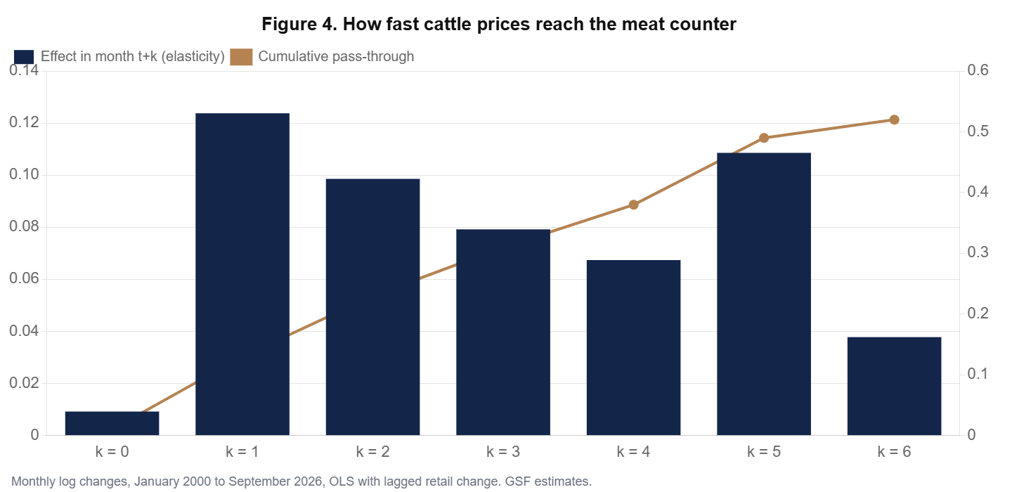
| Cattle price change, same month (k = 0) | 0.009 | 0.034 | 0.01 |
| k = 1 | 0.124 | 0.034 | 0.13 |
| k = 2 | 0.099 | 0.035 | 0.23 |
| k = 3 | 0.079 | 0.034 | 0.31 |
| k = 4 | 0.067 | 0.034 | 0.38 |
| k = 5 | 0.109 | 0.034 | 0.49 |
| k = 6 | 0.038 | 0.034 | 0.52 |
| Retail price change, previous month | -0.179 | 0.056 | |
| Long-run pass-through | 0.445 | ||
| Levels model: elasticity of retail to cattle price | 0.417 | 0.020 | trend +3.4% a year |
Four results stand out (Figure 4). First, there is no contemporaneous pass-through: a cattle price shock in a given month has no measurable effect on retail ground beef in that month. Second, transmission is spread over the following five months, with the largest single effect after one month. Third, about half of a cattle price change reaches the retail price within six months, and the long-run share, once the slight overshooting captured by the negative autoregressive term is taken into account, is about 0.45. The levels model, which relates price levels rather than changes, gives a very similar elasticity of 0.42. Fourth, these shares are well below one because cattle represent only part of the retail price; processing, transport, retail labour and imported lean trim account for the rest.
We also tested for the asymmetry that consumers often suspect, the idea that prices go up like rockets and come down like feathers. We split cattle price changes into increases and decreases and estimated separate coefficients on the sum of each over the previous seven months. The coefficient on increases is 0.054 (standard error 0.021) and the coefficient on decreases is 0.101 (standard error 0.019). If anything, declines in cattle prices have been transmitted more strongly than increases since 2000, although the difference between the two is not large enough to be statistically decisive. The practical message is that the data give no reason to expect retailers to sit on falling cattle costs.
The turning point that retail prices have not yet seen
That finding matters now, because cattle prices have turned. The slaughter cattle index peaked at 408.6 in May 2026 and fell to 346.8 in September, a decline of 15.1% in four months. The reasons include the gradual reopening of the Mexican border, heavier carcass weights, and weaker demand at the very top of the price range. Retail ground beef has not followed: it cost $6.75 in May and $6.76 in October.
Applying the lag structure of Table 2 to the cattle decline already recorded, the pure pass-through effect is a fall of about 8.6% in retail ground beef over the coming months. The estimated constant, which captures the average upward drift of retail prices relative to cattle over 26 years (about 4% a year, reflecting labour, energy and packaging costs), offsets part of it. To show the range of plausible outcomes, we project the retail price under three paths for cattle prices from October 2026 (Figure 5 and Table 3).
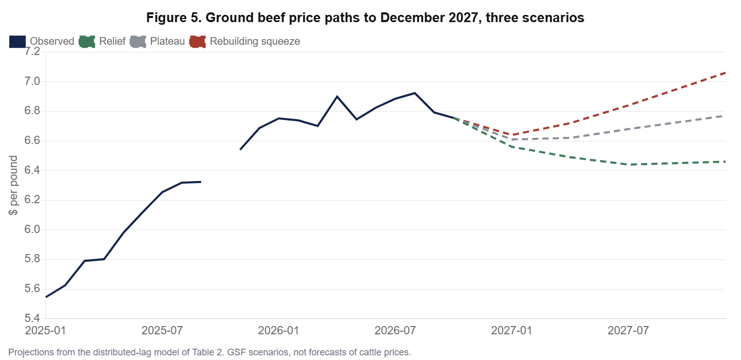
Table 3. Projected retail price of ground beef, $ per pound
| Cattle price scenario | Jan 2027 | Apr 2027 | Jul 2027 | Dec 2027 |
|---|---|---|---|---|
| Relief: cattle prices fall a further 10% by mid-2027 | 6.56 | 6.49 | 6.44 | 6.46 |
| Plateau: cattle prices hold at their September 2026 level | 6.61 | 6.62 | 6.68 | 6.77 |
| Rebuilding squeeze: cattle prices rise 12% by end-2027 | 6.64 | 6.72 | 6.84 | 7.06 |
The three paths agree on the near term. Whatever happens to cattle prices from here, the decline already recorded between May and September should bring ground beef down to roughly $6.55 to $6.65 by January 2027, a fall of 2% to 3% from October. Beyond the winter the paths diverge, and the divergence depends almost entirely on what ranchers do with their heifers. That is the subject of the next section.
The rebuilding premium
The cattle cycle contains a cruel paradox. To produce more beef in the future, ranchers must produce less beef today. Every heifer kept for breeding is a heifer that does not go to a feedlot and then to slaughter. She will calve at about two years of age, and her calf will reach slaughter weight eighteen to twenty-four months later. Herd rebuilding therefore reduces supply for two to three years before it increases it. We call the resulting price effect the rebuilding premium.
To size it, we built a simple supply ledger. The assumptions are explicit and deliberately round: a target expansion of 5% in the beef cow herd (1.38 million head) achieved over two years; carcass weights of about 830 pounds for heifers, 880 pounds for steers and 650 pounds for cull cows; a reduction of 300,000 head in annual cow slaughter as ranchers keep older cows longer; a calving rate of 88%; and a demand elasticity for beef of minus 0.7, in the middle of published estimates. The base is the Department of Agriculture’s estimate of 25.7 billion pounds of US beef production in 2026.
Table 4. Supply ledger of a 5% herd rebuild and the return of Mexican feeders
| Mechanism | Timing | Beef supply effect | Share of output | Price effect |
|---|---|---|---|---|
| Extra heifer retention and fewer cow culls | 2027 to 2028 | -0.77 bn lb a year | -3.0% | about +4.3% |
| Calves from the expanded herd reach slaughter | from 2029 | +1.01 bn lb a year | +3.9% | about -5.6% |
| Mexican feeder imports back to 1 million head | 2027 onward | +0.86 bn lb a year | +3.3% | about -4.7% |
| Argentine quota increase (60,000 t) | immediate | +0.13 bn lb a year | +0.5% | about -0.7% |
The ledger yields three conclusions. First, a determined rebuild would add about 4% to wholesale beef prices in 2027 and 2028, which is exactly the scenario in which our retail projection climbs above $7 by the end of 2027. Second, the full return of Mexican feeder cattle is the single largest short-term source of relief available to policy, roughly equivalent to the supply effect of the rebuild itself. The two would broadly cancel out: a reopened border is what allows ranchers to rebuild without pushing prices higher. Third, the Argentine quota is economically small. Sixty thousand additional tons equal about 0.5% of US production and about 3.4% of the 1.76 million tons the United States imported in the first eleven months of 2025. Its political visibility far exceeds its market weight.
What this means for policy and for inflation
For the administration and the new Congress, the analysis suggests a clear order of priorities. The border matters most in the short run, and the case for a full and predictable reopening, combined with the sterile fly programme that is building a new production plant in Texas, is strong. Measures that make heifer retention easier to finance, such as drought insurance, longer-tenor operating credit for breeding stock and faster disaster payments, act on the structural cause. Competition enforcement should proceed on its own merits, but it should not be sold to households as a remedy for the price of hamburger. Import quotas can help at the margin, at the cost of friction with domestic producers.
For the Federal Reserve, beef is a relative price, not a source of generalised inflation. Beef and veal carry a relative importance of 0.63% in the consumer price index. A 14% to 16% annual increase, as in early 2026, added between 0.065 percentage points (the BLS estimate for February 2026) and about 0.09 points to headline inflation, a non-trivial amount at a time when headline inflation is driven mainly by energy. The decline in cattle prices already recorded should turn that contribution slightly negative in the first half of 2027. It is a small tailwind, not a reason to change the course of policy, but it is one of the few components of the food basket where the direction of the next move is already visible in the data.
For households, the message is less comforting. Even in our most favourable scenario, ground beef ends 2027 at about $6.46 a pound, well above any price seen before 2025. The working-time cost will remain near ten minutes per pound, and the substitution toward chicken, pork and imported lean beef will continue. The cattle cycle can be shortened by good policy but not abolished.
Conclusion
America’s beef prices are high for a reason that is both simple and stubborn: the country has fewer cattle than at any time since the early 1950s, and rebuilding the herd takes years. The data reject the idea that processors captured the increase; since 2023 they have been squeezed between record cattle costs and slower-rising output prices. The data also show that the market transmits cattle price movements to consumers within about six months and in both directions, which means that the 15% fall in cattle prices since May will reach the meat counter this winter. Beyond that, the decisive variable is the herd. If ranchers start to rebuild in earnest, prices will rise again before they fall, unless the Mexican border is fully reopened. Lasting relief belongs to 2029, not to 2027.
Beef is a reminder that some of the most politically charged prices in the American economy are governed by biological lags that no executive order can compress. The best policies are those that work with the cycle rather than against it.
Methodological note
Data: BLS average retail prices for 100% ground beef (APU0000703112), sirloin steak (APU0000703613), whole chicken (APU0000706111) and pork chops (APU0000FD3101); PPI for slaughter cattle (WPU0131) and animal slaughtering except poultry (PCU311611311611); CPI-U all items and food at home; average hourly earnings of all private employees (CES0500000003). All series downloaded from FRED on 11 November 2026. Annual 2026 values are year-to-date averages. Missing monthly observations were interpolated geometrically for the regressions only. The distributed-lag and levels models were estimated by OLS; standard errors are conventional and do not correct for serial correlation, so they should be read as indicative. The supply ledger and price scenarios are illustrative calculations under stated assumptions, not forecasts.
GO DEEPER
The 2026 US Economy Trilogy (3 books, PDF)
Growth from the AI investment boom, the Federal Reserve and the credit economy, and what inflation leaves in the household budget: the forces behind this article, analysed in three research books by Dr. Driss Effina. About 900 pages in English PDF.
$59 instead of $90
Sources
- U.S. Bureau of Labor Statistics, Consumer Price Index news releases (October 2026, February 2026) and CPI relative importance tables; average price data and PPI series via FRED, Federal Reserve Bank of St. Louis.
- USDA National Agricultural Statistics Service, Cattle report, 30 January 2026 and July 2026; USDA WASDE, 2026 beef production estimate.
- American Farm Bureau Federation, Market Intel: Smaller Cattle Herd Creates Market Volatility (2026). Federal Reserve Bank of Kansas City, High Costs and Uncertainty Will Likely Keep Cattle Inventories Low and Beef Prices Elevated for Some Time, 5 August 2026. farmdoc daily, Food Inflation and the Outlook for Beef Prices, 5 October 2026.
- Beef Magazine, U.S./Mexico border opens, 25 August 2026; Associated Press, With tighter checks for flesh-eating screwworm, a border crossing reopens, 26 October 2026; Southern Ag Today, Reopening the Border to Mexican Cattle Imports is the Right Decision, July 2026.
- Reuters, US Justice Department probes meatpackers, November 2025; Western Livestock Journal, Trump calls on DOJ to investigate packers, November 2025; Drovers, U.S. Cattle Inventory Hits 75-Year Low at 86.2 Million Head, January 2026.
- Driss EFFINA, PhD | Independent Researcher, Global Strategy Files | globalstrategyfiles.com
Driss EFFINA, PhD
The opening pages of our four country reports: United States, United Kingdom, Japan and China. A free PDF, sent to your inbox.
You will also receive occasional analysis from Global Strategy Files. Unsubscribe in one click, at any time.