Australia’s Housing Correction in 2026: Interest Rates, Affordability Limits and a Supply Shortage That Has Not Gone Away

Australia’s Housing Correction in 2026: Interest Rates, Affordability Limits and a Supply Shortage That Has Not Gone Away

Driss EFFINA, PhD Independent Researcher, Global Strategy Files Reading time: about 26 minutes

Abstract

Australian dwelling values reached a record high in March 2026 and have fallen in every month since. By September 2026, national values were 5.2 percent below their peak according to the Cotality Home Value Index, with Sydney down 8.6 percent from its February peak and Melbourne down more than 7 percent. This article analyses the correction using data from Cotality, the Australian Bureau of Statistics (ABS) and the Reserve Bank of Australia (RBA), and builds five original indicators: the dispersion of price changes across markets and its relationship with rental yields, the share of income needed to service a new mortgage at successive interest rates, the borrowing capacity of a median income household, the gap between completions and the targets of the National Housing Accord, and a simple estimate of underlying dwelling demand from population growth. The results show that the correction is driven mainly by the four increases in the cash rate in 2026, which reduced the borrowing capacity of a median income household by about 8 percent and pushed the repayment on a new loan for a median value home above half of median household income. The correction is concentrated in the most expensive and lowest yielding markets, while high yield markets such as Perth and Darwin are still rising. At the same time, the supply shortage has not been resolved: completions of about 180,500 dwellings in the year to June 2026 were 25 percent below the pace required by the Accord, rents are still rising by 5.7 percent a year, and the rental vacancy rate remains below 2 percent. The article concludes that Australia is experiencing a credit-driven price correction inside a structural shortage, which limits the depth of the fall but also means that lower prices will not by themselves restore affordability.

Keywords: Australia, housing market, dwelling prices, mortgage serviceability, borrowing capacity, housing supply, National Housing Accord, rents, monetary policy

JEL codes: R21, R31, E43, E52, G21

1. Introduction

For most of the past three decades, Australian housing has been one of the most expensive in the developed world relative to incomes. Episodes of decline have been short and shallow: prices fell in 2008, in 2011 and 2012, in 2017 to 2019, and in 2022, but each time they recovered quickly and went on to new highs. The national median dwelling value rose by about two thirds over the ten years to August 2026.

The current correction began in April 2026, after the national index reached a record high in March. It followed the Reserve Bank of Australia’s decision to reverse the rate cuts of 2025: the cash rate was raised from 3.60 percent to 3.85 percent in February 2026, then to 4.10 percent in March and 4.35 percent in May, and to 4.60 percent at the end of September. The previous article in this series examined the reasons for this tightening. The present article examines its effects on the housing market.

The analysis addresses four questions. How large and how widespread is the correction? Through which channels have higher interest rates affected the market? Has the shortage of housing supply, which has been the dominant theme of Australian housing policy in recent years, been resolved or merely masked? And how far might prices fall?

To answer these questions, the article combines the latest Cotality index data, ABS data on building activity, lending, population and the value of the dwelling stock, and RBA data on interest rates. All derived indicators are the author’s own calculations.

Section 2 sets out the context. Section 3 reviews the literature. Section 4 describes the data and methods. Section 5 presents the results. Section 6 discusses them. Section 7 presents three scenarios to the end of 2027. Section 8 concludes.

2. Context

2.1 A market at a record high

The Australian housing market entered 2026 after a strong year. The three rate cuts of 2025, combined with an expansion of government support for first home buyers and continued population growth, lifted demand. National values rose throughout 2025 and into early 2026, with especially strong gains in Perth, Brisbane and Adelaide, which had been relatively affordable before the pandemic. Over the five years to August 2026, values rose by about 80 percent in Perth and about 64 percent in Brisbane and Adelaide, compared with less than 6 percent in Sydney and a decline in Melbourne.

Affordability had deteriorated to record lows. According to the housing affordability report published by Cotality and the Australian National University in late 2025, the ratio of the national median dwelling value to median household income reached 8.2, it took about eleven years for a household on the median income to save a 20 percent deposit, and servicing a new mortgage required about 45 percent of median household income, against a twenty year average of just over one third. Renters were also under pressure: rent absorbed a record 33.4 percent of median household income.

2.2 The rate shock

The 2026 tightening affected this fragile position directly. The average outstanding variable mortgage rate for owner-occupiers, as published by the RBA, rose from 5.50 percent in January 2026 to 6.20 percent in August, and is expected to reach about 6.45 percent once the September increase has passed through. Because most Australian mortgages are at variable rates, these changes affect both new buyers and existing borrowers within weeks.

Banks also assess borrowers’ capacity to repay at an interest rate at least 3 percentage points above the loan rate, in line with the serviceability buffer set by the Australian Prudential Regulation Authority. Higher rates therefore reduce the maximum amount that a household can borrow, which directly limits what buyers can pay.

2.3 The supply agenda

At the same time, Australian governments have committed to an ambitious supply target. Under the National Housing Accord, the Commonwealth, states and territories agreed to build 1.2 million new well-located homes over five years from 1 July 2024 to 30 June 2029, an average of 240,000 a year or 60,000 a quarter. This target was based on the view that Australia faced a structural shortage of housing, caused by decades of population growth outpacing construction and by planning restrictions that limit supply in the most desirable areas.

2.4 The current correction

Since April 2026, the market has reversed. In September 2026, national values fell by 1.1 percent, the sixth consecutive monthly decline, and were 5.2 percent below their March peak and unchanged over twelve months. Values in the combined capitals were 1.8 percent lower than a year earlier, while regional values were still 5.6 percent higher. Values fell over the three months to September in 97 percent of capital city suburbs.

The ABS confirmed the turn. The total value of Australia’s residential dwellings fell by 0.3 percent, or A$34.1 billion, in the June quarter of 2026, to A$12.7 trillion, the first decline since the September quarter of 2022. The mean dwelling price fell by 0.7 percent to about A$1.1 million, with the largest declines in New South Wales (2.4 percent) and Victoria (2.1 percent).

3. Literature review

Research on Australian housing prices has developed around three main questions.

The first concerns the determinants of prices and whether they are justified by fundamentals. Himmelberg, Mayer and Sinai (2005) proposed comparing the cost of owning with the cost of renting, the user cost approach, rather than relying on price to income ratios, which ignore interest rates. Fox and Tulip (2014), applying this approach to Australia, concluded that the rise in prices up to the early 2010s was largely explained by the fall in interest rates. Saunders and Tulip (2019), in a model developed at the RBA, showed that interest rates are the dominant driver of fluctuations in Australian housing prices in the short and medium term, and estimated that each 1 percent increase in the stock of dwellings reduces prices and rents by about 2.5 percent.

The second concerns the role of supply and planning. Glaeser and Gyourko (2018) showed that in the United States, high prices in many cities reflect restrictions on supply rather than high construction costs. Kendall and Tulip (2018), in an RBA research paper, estimated that zoning and planning restrictions add a large premium to the price of detached houses in Australian capitals, especially in Sydney and Melbourne. The Productivity Commission (2025), in its report on housing construction productivity, found that the productivity of housing construction in Australia fell by about 12 percent over thirty years, while productivity in the economy as a whole rose by about 49 percent, which helps explain why supply responds slowly to demand.

The third concerns the transmission of monetary policy through housing. La Cava, Hughson and Kaplan (2016) showed that the large share of variable rate mortgages makes Australian households’ spending particularly sensitive to changes in interest rates. The RBA’s Financial Stability Reviews regularly assess the resilience of borrowers to rate increases and price declines.

The present article contributes to this literature by measuring the 2026 correction with current data, by quantifying the effect of interest rates on serviceability and borrowing capacity at each stage of the tightening, and by showing that the correction is concentrated in low yield markets, which is consistent with the user cost approach.

4. Data and methodology

4.1 Data

The data come from:

• the Cotality Home Value Index for August and September 2026, which gives monthly, quarterly and annual changes in dwelling values, peak to date changes, gross rental yields, median values, rents, vacancy rates, sales and listings for capital cities and regional areas;
• the ABS releases on Building Activity (June quarter 2026), Building Approvals (August 2026), Lending Indicators (June quarter 2026), National, State and Territory Population (March quarter 2026), Total Value of Dwellings (June quarter 2026) and Average Weekly Earnings (May 2026);
• RBA Table F6 on housing lending rates and the RBA’s statements of September 2026;
• the Cotality and Australian National University housing affordability report of late 2025, for median household income.

4.2 Indicators

The author calculates:

1. Dispersion and yield relationship. For the eight capitals and six regional areas covered by the Cotality index, the author compares the annual change in values with the gross rental yield and with the change over five years, and computes simple correlation coefficients and a fitted linear relationship. 2. Mortgage serviceability. The monthly repayment on a 30-year principal and interest loan equal to 80 percent of the national median dwelling value (A$912,885 in August 2026, so a loan of about A$730,000) is calculated at five interest rates: 5.50, 6.20, 6.45, 6.70 and 6.95 percent. The annual repayment is expressed as a share of median household income. Median household income for 2026 is estimated by applying growth of 4 percent to the September 2025 figure of A$104,390, giving about A$108,600. This assumption is consistent with growth in average weekly earnings of 3.7 percent over the year to May 2026. 3. Borrowing capacity. The maximum loan for a household on the median income is calculated assuming that repayments may not exceed 30 percent of gross income, assessed at the loan rate plus 3 percentage points. This is a simplified version of bank serviceability models, which also take into account living expenses, other debts and tax. 4. Accord progress. Completions in the first two years of the Accord are compared with the target, and the annual pace required to reach 1.2 million by June 2029 is calculated. 5. Underlying demand. New demand for dwellings is estimated as the annual increase in the population divided by an average household size of 2.5 persons, plus the replacement of 0.3 percent of the dwelling stock each year. The stock is estimated at about 11.5 million dwellings by dividing the ABS total value of dwellings by the mean dwelling price.

4.3 Limitations

The Cotality index measures the value of the whole stock using a hedonic method; it is not the same as the median sale price. The serviceability and borrowing capacity calculations are stylised and apply to a household on the median income buying the median home, a situation that does not describe every buyer. The demand estimate is sensitive to the assumed household size: a lower household size, as has been observed in periods of strong income growth, raises demand. The scenarios are illustrative.

5. Results

5.1 The scale and geography of the correction

Figure 1 shows the change in dwelling values in the eight capital cities over the twelve months to August 2026 and the decline from each city’s cyclical peak.

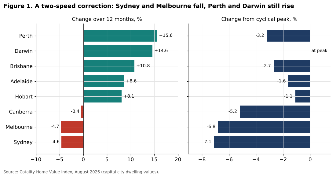
The first result is the divergence between markets. Over the twelve months to August 2026, values fell by 4.6 percent in Sydney and 4.7 percent in Melbourne, and were broadly unchanged in Canberra. In the other capitals they were still rising strongly: by 15.6 percent in Perth, 14.6 percent in Darwin, 10.8 percent in Brisbane, 8.6 percent in Adelaide and 8.1 percent in Hobart. Regional areas also recorded gains, from 4.6 percent in regional Victoria to 16.7 percent in regional Western Australia.

However, the decline from the peak shows that the correction is spreading. By August, Sydney values were 7.1 percent below their February peak, Melbourne 6.8 percent below its March 2022 record, Canberra 5.2 percent below its May 2022 record, Perth 3.2 percent below its April 2026 peak and Brisbane 2.7 percent below its May 2026 peak. Only Darwin and regional South Australia were still at their peak. In September, the decline accelerated: Sydney fell by 1.4 percent in the month and Brisbane by 1.5 percent, and Sydney was 8.6 percent below its peak.

Market	Change over 12 months	Change from peak	Change over 5 years	Gross yield	Median value
Sydney	-4.6%	-7.1%	+5.6%	3.3%	A$1,222,718
Melbourne	-4.7%	-6.8%	-3.9%	4.0%	A$786,718
Brisbane	+10.8%	-2.7%	+64.1%	3.4%	A$1,080,142
Adelaide	+8.6%	-1.6%	+64.0%	3.6%	A$937,207
Perth	+15.6%	-3.2%	+79.7%	3.9%	A$999,987
Hobart	+8.1%	-1.1%	+11.5%	4.4%	A$752,397
Darwin	+14.6%	at peak	+30.6%	6.3%	A$647,259
Canberra	-0.4%	-5.2%	+6.3%	4.3%	A$864,998
National	+2.7%	-3.6%	+23.9%	3.8%	A$912,885

Table 1. Dwelling values in August 2026. Source: Cotality Home Value Index.

The volume of transactions has fallen more sharply than prices. Cotality estimates that home sales in the three months to September 2026 were 19.1 percent lower than a year earlier and 13.3 percent below the five-year average, with declines of more than 25 percent in Brisbane and Sydney. Total listings in the capitals were 23.1 percent higher than a year earlier, while new listings were 9.2 percent lower: fewer people are putting their homes on the market, but those that are listed take longer to sell. The median time to sell in the capitals rose from 23 days a year earlier to 39 days.

This combination, more stock on the market and fewer buyers, is typical of the early stage of a correction. It indicates that the adjustment is driven by demand, not by forced sales: owners are not under pressure to sell, which limits the speed of the price decline.

5.2 The credit channel: serviceability and borrowing capacity

Figure 2 shows the effect of higher interest rates on the affordability of a new mortgage for a median income household buying a median value home.

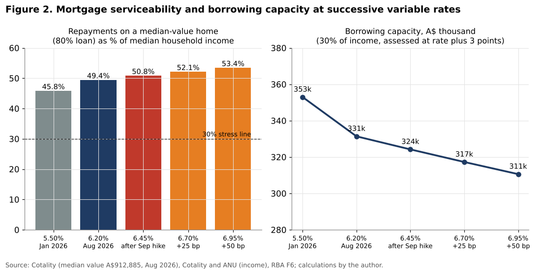
The left panel shows the annual repayment on a loan of about A$730,000 as a share of estimated median household income. At the average variable rate of January 2026 (5.50 percent), it was 45.8 percent, consistent with the 45 percent estimated by Cotality and the ANU for 2025. At 6.20 percent (August 2026), it rises to 49.4 percent, and after the September increase (6.45 percent), to 50.8 percent. If the cash rate were raised once more, the share would reach 52.1 percent, and with two more increases, 53.4 percent.

In other words, for the first time, servicing a new loan on a median value home requires more than half of the gross income of a median income household. A common benchmark of housing stress is a housing cost above 30 percent of income. At current rates, a median income household cannot buy a median value home without being far above this benchmark.

The right panel shows the borrowing capacity of the same household, on the simplified assumption that banks allow repayments of up to 30 percent of gross income, assessed at the loan rate plus 3 percentage points. Borrowing capacity falls from about A$353,000 at the January 2026 rate to about A$324,000 after the September increase, a fall of 8.2 percent. This is very close to Cotality’s estimate that the four increases of 2026 reduced the borrowing capacity of a typical household by almost A$90,000, or about 9 percent, for a higher income household.

The gap between borrowing capacity and prices is striking. A household on the median income, assessed in this conservative way, can borrow only about A$324,000, while a 20 percent deposit on the median home would require a loan of about A$730,000. In practice, buyers bridge this gap through two incomes above the median, larger deposits (often with family help), government guarantee schemes for first home buyers, or by buying cheaper homes. But the reduction in borrowing capacity in 2026 directly lowers the maximum price that the marginal buyer can pay, and it is this effect, rather than any increase in forced sales, that drives the correction.

The ABS lending data confirm this mechanism. In the June quarter of 2026, the number of new loan commitments for dwellings fell by 5.4 percent from the previous quarter, to 134,225. Owner-occupier commitments fell by 3.3 percent in number and 1.9 percent in value, to A$60.5 billion. Investor lending fell more sharply, by 10.2 percent in value to A$37.1 billion, and its annual growth slowed from 19.4 percent in the March quarter to 2.8 percent. First home buyers were the most resilient group: the number of their loans fell by 2.9 percent, while the value was broadly stable at A$18.4 billion, supported by government schemes.

5.3 The supply shortage has not been resolved

Figure 3 compares dwelling completions with the National Housing Accord target.

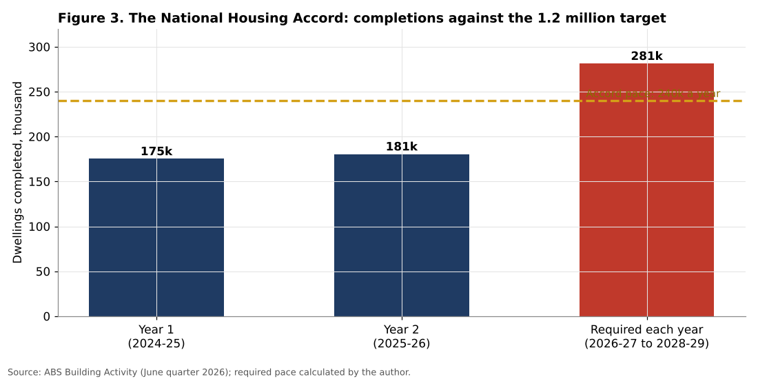
In the first year of the Accord (July 2024 to June 2025), about 175,300 dwellings were completed. In the second year (July 2025 to June 2026), completions rose to about 180,500. The total for the first two years, 355,817, is 124,183 short of the pro rata target of 480,000, a shortfall of 26 percent. To reach 1.2 million by June 2029, about 281,400 dwellings would need to be completed each year in the remaining three years, 56 percent more than in 2025 to 2026. The highest quarterly completion figure since the series began in 1984 is about 58,800, which corresponds to an annual pace of about 235,000. Reaching the Accord target would therefore require an unprecedented level of activity for three consecutive years.

There are some positive signs. Completions in the June quarter of 2026 (47,168, seasonally adjusted) were 15.9 percent higher than a year earlier, and commencements (52,201) were 14.4 percent higher. The number of dwellings under construction reached a record of 248,733, above the previous high of September 2022. At the current rate of completions, this pipeline represents about 1.4 years of work. Approvals for private houses in August 2026 were 18.4 percent higher than a year earlier.

But the pipeline is slow to convert into homes. Apartments take on average more than two years to complete. Approvals for apartments and townhouses fell sharply in August 2026 (by 21.2 percent in the month for private dwellings other than houses), and the fall in prices, combined with high construction costs and higher interest rates, reduces the profitability of new projects. The Productivity Commission’s finding that housing construction productivity has declined over three decades suggests that the industry’s capacity to accelerate is limited.

5.4 Demand and supply

Figure 4 compares an estimate of underlying new demand with completions and the Accord pace.

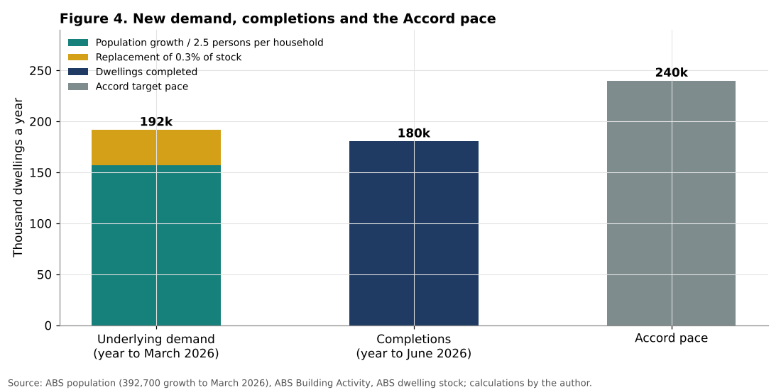
Australia’s population grew by 392,700, or 1.4 percent, in the year to March 2026, to 27.9 million. Net overseas migration accounted for 292,100 and natural increase for 100,600. With an average household size of 2.5 persons, this population growth implies demand for about 157,000 additional dwellings. Adding the replacement of 0.3 percent of the stock of about 11.5 million dwellings, about 35,000 a year, gives total underlying demand of about 192,000 dwellings a year.

Completions in the year to June 2026, about 180,500, were therefore about 11,000 below underlying demand on this estimate. The gap is much smaller than in 2023 and 2024, when population growth exceeded 2 percent a year and completions were lower, but it has not closed. The accumulated shortfall of previous years has not been absorbed.

This explains a central paradox of the current correction: prices are falling, but rents are still rising. In August 2026, Cotality’s national rent index was 5.7 percent higher than a year earlier, and rents have risen by 39 percent over five years. The national rental vacancy rate was 1.9 percent, slightly above the record low of 1.5 percent reached in February 2026, but still well below the 3 percent generally regarded as a balanced market. The shortage of homes continues to be expressed in the rental market, while the correction in prices reflects the fall in borrowing capacity.

The Accord shortfall of about 124,000 dwellings represents about 1.1 percent of the dwelling stock. Using the elasticity estimated by Saunders and Tulip (2019), according to which each 1 percent increase in the stock reduces prices and rents by about 2.5 percent, this shortfall corresponds to housing costs about 2.7 percent higher than they would have been if the Accord pace had been achieved. This is a modest effect in relation to the effect of interest rates, which confirms that supply policies, while necessary, act slowly and cannot offset large changes in the cost of credit.

5.5 Where the correction bites: yields and price changes

Figure 5 shows the relationship between gross rental yields and the change in values over twelve months for the fourteen markets covered by the Cotality index.

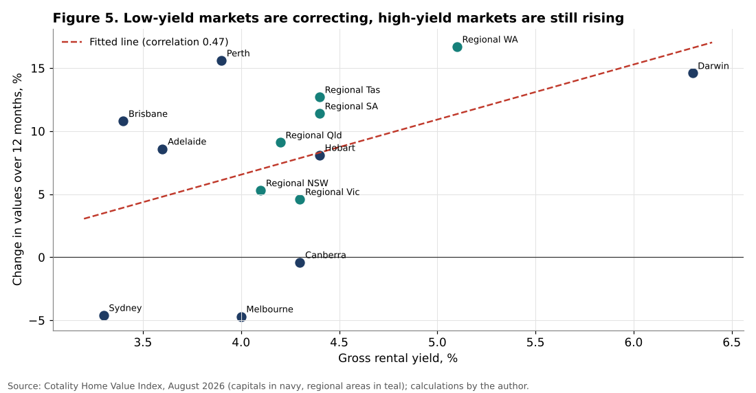
There is a positive relationship between yields and price growth: markets with higher rental yields recorded larger price increases. The correlation coefficient is 0.47 and the fitted line implies that each additional percentage point of gross yield is associated with about 4.4 percentage points more growth in values over the year. Sydney, with the lowest yield (3.3 percent), recorded one of the largest falls. Darwin, with the highest yield (6.3 percent), and regional Western Australia (5.1 percent) recorded among the largest increases.

This result is consistent with the user cost approach. When interest rates rise, the cost of owning a home rises relative to the cost of renting it. The increase in the cost of ownership is proportionally larger in markets where the rental yield is low, because a larger part of the expected return comes from capital gains rather than rent. These markets are therefore the most exposed to rate increases.

The relationship with past growth is even stronger. The correlation between the change in values over five years and the change over the past twelve months is 0.79: markets that had grown strongly over five years (Perth, Brisbane, Adelaide, regional Western Australia and regional South Australia) continued to grow over the past year, while those that had stagnated (Sydney, Melbourne, Canberra) declined. This persistence reflects both momentum and differences in affordability: in 2021, Perth and Brisbane were much cheaper than Sydney and Melbourne, which allowed them to absorb a larger share of demand. Since then, the gap has narrowed considerably: Brisbane’s median value (about A$1.08 million) now exceeds Melbourne’s (about A$0.79 million) by more than a third, and Perth’s (about A$1.0 million) is approaching Sydney’s lower segments.

The monthly data for September suggest that the correction is now spreading to the cities that had been most resilient. Brisbane recorded the largest monthly fall (1.5 percent), and Perth, Adelaide and the other mid-sized capitals all fell by more than 1 percent. Only Darwin rose.

5.6 Household balance sheets

The correction does not appear to threaten household balance sheets or the financial system in the short term. According to the RBA, scheduled mortgage payments represent about 10 percent of household disposable income, close to the 2024 peak. Less than 2 percent of owner-occupier borrowers face a cash flow shortfall, arrears are low, and negative equity would remain rare even if prices fell by 20 percent. Household debt has fallen relative to income, from about 187 percent of disposable income in 2019 to about 178 percent in mid-2026.

These figures reflect the large equity cushion built up by most owners during the price increases of recent years. A household that bought five years ago has, on average, seen the value of its home rise by about a quarter nationally, and by much more in Perth, Brisbane and Adelaide. A fall of 5 to 10 percent wipes out only part of these gains.

The most exposed borrowers are recent buyers in Sydney and Melbourne, who bought near the peak with high loan to value ratios, and investors who rely on capital gains rather than rent to cover their costs. The sharp fall in investor lending in the June quarter of 2026 suggests that this group is already adjusting.

6. Discussion

6.1 A correction driven by credit, not by a collapse of demand

The evidence presented in this article indicates that the 2026 correction is primarily a credit-driven adjustment. Four rate increases have reduced borrowing capacity by about 8 percent, which corresponds closely to the 5 to 9 percent fall in values from the peak in the most affected markets. The correction is concentrated where yields are lowest and prices relative to incomes are highest, which is what the user cost approach predicts.

Underlying demand has not collapsed. Population growth remains at 1.4 percent a year, the rental market remains tight, and rents are still rising faster than incomes. This is a crucial difference with corrections caused by an excess of supply, as in the United States after 2006 or in China today, analysed in an earlier article in this series. In Australia, there is no overhang of vacant homes; on the contrary, there is a shortage.

6.2 The limits of the correction

This configuration sets limits on the depth of the correction. As prices fall and rents rise, rental yields increase, which makes investment more attractive and slows the decline. The large equity buffers of most owners mean that there are few forced sales. And the supply shortage means that the stock of available homes does not grow fast enough to push prices down sharply.

Historical experience supports this conclusion. In the 2017 to 2019 correction, driven by tighter lending standards, national values fell by about 8 percent and Sydney values by about 15 percent. In the 2022 to 2023 correction, driven by the rapid increase in interest rates from 0.10 to 4.35 percent, national values fell by about 9 percent before recovering. Both corrections ended when credit conditions eased.

6.3 Affordability is not restored

A fall in prices does not mean that affordability improves. Because the fall is caused by higher interest rates, the cost of buying a home, measured by repayments as a share of income, has risen even as prices have fallen. The share of income required to service a new loan on the median home has increased from about 46 percent to about 51 percent since January 2026, despite the fall in values.

For renters, the situation has not improved either. Rents continue to rise by more than 5 percent a year, faster than wages. And for those saving a deposit, the fall in prices is too small to make a meaningful difference.

The only lasting improvement in affordability would come from a combination of lower interest rates, which depend on inflation, and a sustained increase in supply. The first is not on the immediate horizon, as the previous article in this series showed. The second is progressing, but much more slowly than the Accord target requires.

6.4 The risk to supply

The correction poses a specific risk to the supply agenda. Housing construction, particularly of apartments, depends on presales and on the expectation of stable or rising prices. When prices fall and construction costs remain high, many projects become unprofitable and are delayed or cancelled. The sharp fall in apartment and townhouse approvals in August 2026 is an early warning sign. The RBA Governor noted in September that a downturn combined with high building costs could discourage development, worsening the structural shortage in the medium term.

This creates a potential cycle: higher rates lower prices, lower prices reduce construction, reduced construction worsens the shortage, and the shortage pushes rents and eventually prices up again when rates fall. Breaking this cycle requires policies that raise the productivity of construction and reduce the cost and delay of planning approvals, so that supply can respond to demand at a lower price.

6.5 Policy implications

Several implications follow from the analysis.

First, the RBA is right to judge that the housing correction does not threaten financial stability. Borrowers have large equity buffers, and the correction is driven by reduced demand rather than distressed sales.

Second, governments should be cautious about responding to falling prices with new demand subsidies for first home buyers. Such measures increase borrowing capacity and therefore prices, offsetting part of the effect of monetary policy, without increasing supply.

Third, the supply agenda needs to focus on productivity and approval processes rather than on headline targets. The Accord target is unlikely to be met, and the gap between required and actual completions is too large to be closed by incremental measures.

Fourth, the rental market requires specific attention. Rents are rising faster than incomes, and renters do not benefit from falling prices. Policies that encourage institutional investment in rental housing (build to rent) and social housing construction could help.

7. Scenarios to the end of 2027

7.1 Assumptions

Figure 6 presents three scenarios for national dwelling values from September 2026 to December 2027, expressed as an index with the March 2026 peak equal to 100. In September 2026, the index stood at 94.8.

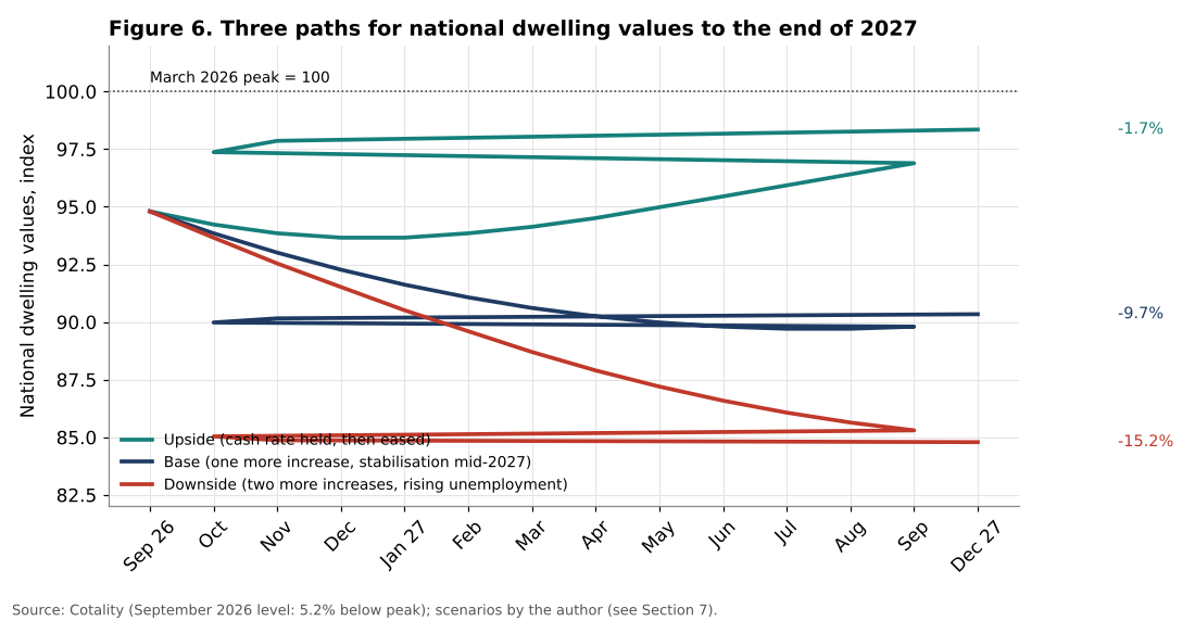
Upside scenario: cash rate held, then eased. The September quarter CPI shows that inflation is stabilising, and the RBA holds the cash rate at 4.60 percent before easing in the second half of 2027. Monthly declines slow quickly, from 0.6 percent in October to zero in January 2027, and values begin to recover modestly from February 2027. The trough is about 6.3 percent below the March 2026 peak, and values end 2027 about 1.7 percent below the peak.

Base scenario: one more increase, stabilisation in mid-2027. The RBA raises the cash rate once more, to 4.85 percent, in November 2026, and holds it through 2027. Monthly declines slow gradually from about 1 percent to zero by mid-2027. Values bottom out at about 10 percent below the peak in the second half of 2027.

Downside scenario: two more increases and rising unemployment. The RBA raises the cash rate twice, to 5.10 percent, and unemployment rises above 5 percent. Declines of about 1 percent a month continue until mid-2027 and slow only gradually. Values are about 15 percent below the peak at the end of 2027.

7.2 Interpretation

The base scenario implies a total correction of about 10 percent, comparable to those of 2017 to 2019 and 2022 to 2023. This is consistent with the reduction of about 8 to 9 percent in borrowing capacity caused by the 2026 tightening, plus a further increase in rates. The downside scenario would produce the largest national correction in decades, but even then, the fall would be smaller than the gains of the past five years in most markets, and the RBA’s stress tests suggest that the financial system could absorb it.

In all three scenarios, the correction would be uneven. The largest declines would be expected in Sydney and Melbourne and, in the base and downside scenarios, in Brisbane, where values rose most rapidly and yields are low. The smallest declines would be expected in Darwin, Perth and regional areas with high yields.

In none of the scenarios does the correction resolve the supply shortage. Even in the downside scenario, rents would continue to rise, because the underlying demand for dwellings, driven by population growth, would continue to exceed completions.

7.3 Indicators to monitor

The author suggests monitoring:

1. the Cotality monthly index, particularly the monthly change in Sydney, Melbourne and Brisbane; 2. the ABS lending indicators, especially investor lending and first home buyer loans; 3. the September quarter CPI and the RBA’s decisions in November and December 2026; 4. rental vacancy rates and rent growth; 5. dwelling approvals for apartments and townhouses, the leading indicator of future supply.

8. Conclusion

This article has analysed the Australian housing correction of 2026 using the latest data from Cotality, the ABS and the RBA. Its main findings are:

1. National dwelling values fell by 5.2 percent from their March 2026 peak to September 2026, with larger falls in Sydney (8.6 percent from its peak) and Melbourne, while Perth, Darwin and regional areas were still higher than a year earlier. 2. The correction is driven by credit. The four rate increases of 2026 raised the repayment on a new loan for the median home from about 46 percent to about 51 percent of median household income and reduced the borrowing capacity of a median income household by about 8 percent. 3. The correction is concentrated in markets with low rental yields, consistent with the user cost approach. The correlation between yields and annual price changes across fourteen markets is 0.47. 4. The supply shortage has not been resolved. Completions of about 180,500 in the year to June 2026 were 25 percent below the Accord pace and below estimated underlying demand of about 192,000. Rents are still rising by 5.7 percent a year. 5. Household balance sheets are strong, and the correction does not threaten financial stability.

The overall conclusion is that Australia is experiencing a credit-driven price correction inside a structural shortage. This combination limits the depth of the price fall, because demand for housing remains strong and owners are not forced to sell. But it also means that lower prices will not by themselves restore affordability. Only a sustained increase in supply, made possible by higher construction productivity and faster approvals, combined with a return of inflation to target and lower interest rates, can achieve that. In the meantime, there is a risk that the correction itself will slow construction and make the shortage worse.

Frequently asked questions

Methodological note

All indicators and scenarios in this article were calculated by the author. Market data come from the Cotality Home Value Index for August 2026 (city tables) and September 2026 (headline results). ABS data come from Building Activity (June quarter 2026), Building Approvals (August 2026), Lending Indicators (June quarter 2026), National, State and Territory Population (March quarter 2026), Total Value of Dwellings (June quarter 2026) and Average Weekly Earnings (May 2026). Interest rates come from RBA Table F6. Median household income for 2026 is an estimate. Serviceability uses the standard annuity formula for a 30-year loan of 80 percent of the national median value; borrowing capacity assumes a maximum repayment of 30 percent of gross income assessed at the loan rate plus 3 points. Underlying demand assumes 2.5 persons per household and replacement of 0.3 percent of the stock. The scenarios are illustrative and do not constitute forecasts or financial advice.

References

Australian Bureau of Statistics (2026). Building Activity, Australia, June 2026; Building Approvals, Australia, August 2026; Lending Indicators, June quarter 2026; National, State and Territory Population, March 2026; Total Value of Dwellings, June quarter 2026; Average Weekly Earnings, Australia, May 2026. Canberra.

Cotality (2026). Home Value Index, August and September 2026. Sydney.

Cotality and Australian National University (2025). Housing Affordability Report. November 2025.

Fox, R. and Tulip, P. (2014). Is Housing Overvalued? Reserve Bank of Australia Research Discussion Paper 2014-06.

Glaeser, E. and Gyourko, J. (2018). The Economic Implications of Housing Supply. Journal of Economic Perspectives, 32(1), 3 to 30.

Himmelberg, C., Mayer, C. and Sinai, T. (2005). Assessing High House Prices: Bubbles, Fundamentals and Misperceptions. Journal of Economic Perspectives, 19(4), 67 to 92.

Kendall, R. and Tulip, P. (2018). The Effect of Zoning on Housing Prices. Reserve Bank of Australia Research Discussion Paper 2018-03.

La Cava, G., Hughson, H. and Kaplan, G. (2016). The Household Cash Flow Channel of Monetary Policy. Reserve Bank of Australia Research Discussion Paper 2016-12.

Productivity Commission (2025). Housing Construction Productivity: Can We Fix It? Research Paper. Canberra.

Reserve Bank of Australia (2026). Statement by the Monetary Policy Board and Minutes of the Monetary Policy Meeting, 29 September 2026; Statistical Table F6, Housing Lending Rates. Sydney.

Saunders, T. and Tulip, P. (2019). A Model of the Australian Housing Market. Reserve Bank of Australia Research Discussion Paper 2019-01.