China Electricity Rationing and Fiscal Borders

Driss EFFINA, PhD Independent Researcher, Global Strategy Files Decoded, China series, 23 October 2026.
A fiscal criterion in a county plan does not establish an executed fiscal distortion. This preview first states the observed policy and the conditional model setup, then presents the fixed-origin zero, a positive flexibility illustration and its disconfirmations. Every power, capacity and fiscal-response parameter remains exposed.
Wuyi makes a fiscal and evaluation gradient visible
Wuyi’s Development and Reform Bureau signed the retained winter load-management plan on 29 October 2024. Search and PDF title metadata misleadingly identify 2013, but the actual cover and signature identify 2024. The original nine-page document is preserved, so the article follows the dated contents rather than the misleading metadata. It is a selected county case linked institutionally to Zhejiang, not a nationally representative policy sample or a record of the 2021 episode discussed in the closest paper. (Wuyi: original 2024 winter load-management plan)
Its first four parcel classes require tax yield above RMB50,000 per mu, differentiated by the lowest enterprise evaluation grade on the parcel: all A, lowest B, lowest C or lowest D. The fifth class is at or below the threshold, and the sixth covers unassessed enterprises or missing parcel correspondence. Parcels are ordered within classes by descending tax yield, with protected enterprises excepted. The rule combines land-based tax yield and evaluation grades; it is not a clean assignment on tax alone. (Wuyi: original 2024 winter load-management plan)
The object classified can be a parcel or supply-settlement account containing multiple enterprises. A parcel’s gross tax yield per unit of land differs from the marginal retained revenue produced by another MWh at one plant. This prevents direct conversion of the threshold into the model’s local objective. Nevertheless, the rule is informative: a fiscal measure appears explicitly in a planned allocation hierarchy. Figure 3 reconstructs the calendar for that hierarchy without pretending to observe individual executed cuts or the customers behind each enterprise’s output.
The distinction leaves a testable question. Conditional on a supplier’s own evaluation, retained tax contribution, protection status and physical constraints, does serving outside customers change actual curtailment? The plan cannot answer it because the named enterprise rosters and several sequence attachments are not included in the retained PDF. The appropriate use of the document is to define potential institutional variables and a transparent planned priority measure. An unobserved roster, dispatch log or customer graph is left missing instead of being reconstructed from broad provincial accounting.
The model setup separates data from every assumed margin
The conditional program has ten production nodes: two origins for each of agriculture/resources, manufacturing/repair, utilities, construction and services. Historical gross output, domestic shipments and total value added come from the verified 2017 aggregation. One common currency scaling makes gross output sum to 100; national value added is separately normalized to an index of 100 at baseline. The exercise does not use contemporary firm customers, actual county retained taxes or a calibrated 2026 grid. Table 5 distinguishes the historical inputs from the numerical assumptions.
Assumed normalized power requirements are 1, 3, 1.5, 0.5 and 0.3 per output unit across the five products, repeated in both regions. They are not measured kWh per RMB. A central 25% power shortage applies to Zhejiang’s modeled discretionary budget, after protected loads are presumed served. The other aggregate region has its baseline budget. Output headroom, origin flexibility, route limits and power links are separately varied. None is fitted to annual national consumption or inferred from the existence of cross-provincial electricity trade.
The national objective counts historical value added wherever it occurs. The local proxy counts Zhejiang value added with an illustrative common weight and assigns zero weight to value added elsewhere. Each is normalized at its own baseline. This is a declared difference in recipients, not an estimated preference, statutory tax rate or claim that an actual authority ignores outside welfare. A mixed-objective parameter traces intermediate weights. At the local endpoint a small national regularizer makes the tie convention explicit, with its possible local sacrifice separately bounded.
Every national-local comparison uses the same feasible set: the same input requirements, origin bounds, power budgets, capacities, terminal-demand caps, routes and transfer losses. Only the objective changes. The national value-added difference is then a conditional opportunity cost of that objective change. This setup must precede its quantitative results. The highlighted flexible illustration uses 10% headroom and 10% origin flexibility; positive headroom is not necessary for every positive grid case. Solver precision cannot supply evidence for these assumptions, and the article does not relabel the resulting index-point gap as an observed Chinese fiscal loss.
Table 5. Historical inputs and exposed assumptions
| Input | Value / treatment | Evidence status |
|---|---|---|
| Domestic IO / total VA | Verified 2017 aggregation | Historical estimated provincial network |
| Power intensities | 1 /3 /1.5 /0.5 /0.3 | Assumed normalized units; not kWh/RMB |
| Shortage / headroom | 25% /0% or 10% central comparisons | Assumed, not observed plant capacity |
| Origin flexibility | 0 to 1 within broad products | Not an estimated elasticity |
| Local fiscal proxy | Own-region VA weight 1; outside 0 | No measured marginal retained tax |
| Transfers / routes | Separate caps; 5% power loss | Assumed physical limits |
Every objective pair shares the same feasible set. No parameter is fitted to a national consumption trend.
Fixed origins eliminate the tested fiscal tradeoff
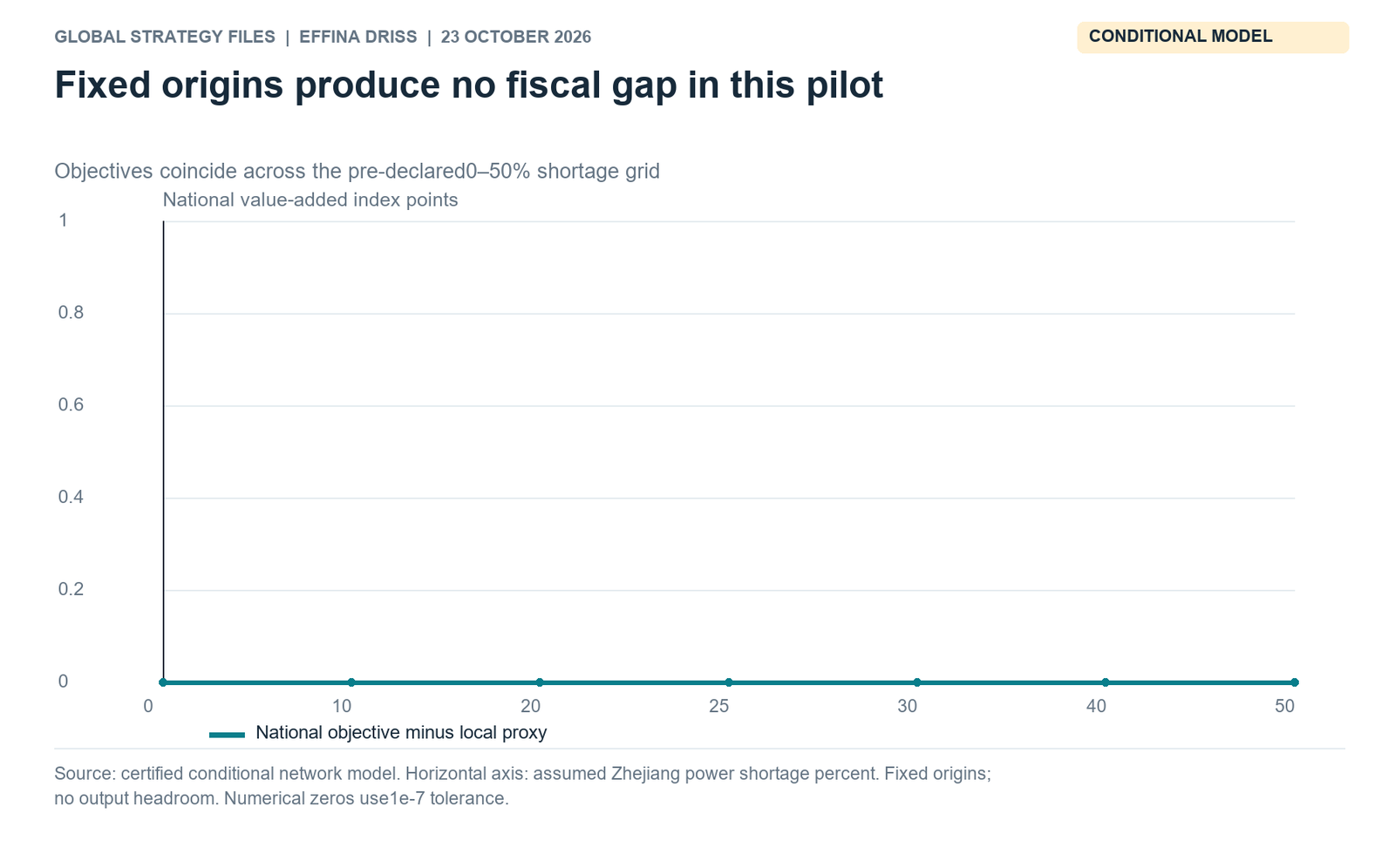
With kappa zero and no output headroom, the national and local endpoints yield the same national allocation index across the tested shortage grid. At the assumed 25% Zhejiang shortfall, the respective results are 98.6894813500 and 98.6894813500, differing only in floating-point rounding. Figure 9 shows the national opportunity-cost gap as zero for shortages of 0, 10, 20, 25, 30, 40 and 50%. Numerical zero means an absolute gap below 10^-7 index points, not that the economy experiences no shortage loss.
At the 25% shortage the national index is about 1.310519 points below baseline, while the local proxy is approximately 86.884068 against its own baseline of 100. Those are different quantities with different normalizations. The first compares national value added with national baseline; the second compares Zhejiang value added with Zhejiang baseline. Their numerical distance cannot be interpreted as a fiscal-border wedge. The wedge compares national value added under two objectives facing the same constraints, and in this benchmark that difference is zero.
This result is stronger than an assertion that borders sometimes matter less. Historical outside sales are present, and local and national objective weights differ, yet the feasible production system supplies no tested alternative yielding a positive national gap. Complementarity, capacity ceilings and fixed origins can make the objectives select the same outcome. The calculation does not prove a universal theorem for every fixed-input economy; it is a certified result for this retained aggregation and tested grid. Its value is to reject a necessary distortion inferred solely from outside links and local weights.
A positive hypothesis must therefore identify an actual discretionary margin. It cannot simply show that a supplier sells outside, that national power use rises, or that a county uses a fiscal classification. Without feasible replacement or reallocation, different interests need not produce different allocations. Conversely, a zero model wedge says nothing about equal household welfare, technical damage or executed policy. It narrows one defined comparison: at the stated historical coefficients and assumptions, replacing the national objective with the local proxy does not further reduce the national index.
A flexible-origin example produces a positive gap
Allow 10% origin flexibility and 10% output headroom, keep the assumed 25% Zhejiang shortage, and compare the same two objectives under the same new constraints. The national endpoint gives 99.040558, while the local endpoint gives 98.776116. Their difference is 0.264442 national value-added index points. This is a selected positive illustration from the fully reported parameter grid. It is not an estimated distortion, a budget amount, a percentage of 2026 GDP or a national lower bound on administrative losses.
The comparison does not hold national output fixed while moving fiscal revenue. It permits alternative feasible production and sourcing choices, then values their historical output contributions. The local proxy can prefer a higher own-region index while preserving less national value added. Neither endpoint is called observed behavior. A welfare interpretation would require further choices about final-use weights, employment, distribution, externalities and dynamic costs that this declared national-value-added criterion does not provide. The positive result demonstrates the possibility of an objective tradeoff within a constrained accounting system.
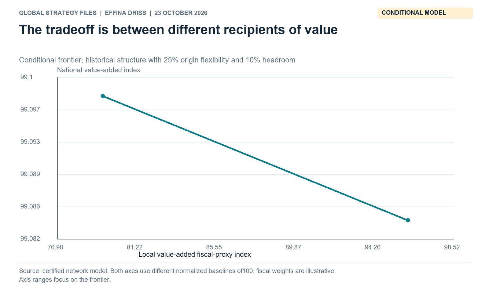
Figure 10 traces mixed objectives at 25% origin flexibility and 10% headroom, a different explicitly labeled case whose endpoint gap is only 0.014150 points. The two plotted axes have their own baselines of 100 and deliberately focused ranges. Their slope is not a tax rate or a fiscal multiplier. Presenting that frontier alongside the larger 10% flexibility example prevents a reader from treating the highlighted 0.264442 as an invariant structural coefficient or confusing two separate parameter settings.
The empirical interpretation remains open in both cases. Actual spare capacity could be unavailable, broad products incompatible, inter-area routes congested or local weights offset by strategic protection. Each issue could remove or alter the modeled tradeoff. That is why the article exposes the fixed-origin zero before the positive example and retains all grid points. A useful mechanism result specifies the conditions that make it possible and the observations that would reject those conditions; decimal precision alone cannot turn the example into evidence of fiscal intent.
More substitution need not shrink the gap monotonically
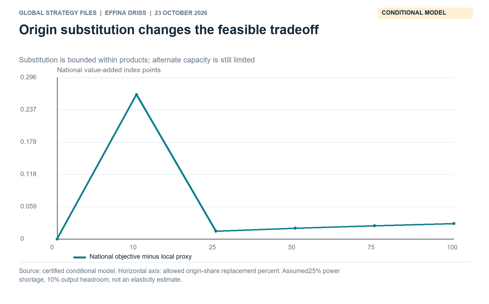
At 10% output headroom and the assumed 25% shortage, the national-local gap for origin-flexibility values 0, 0.10, 0.25, 0.50, 0.75 and 1 is 0, 0.264442, 0.014150, 0.019698, 0.024377 and 0.028371 index points. Figure 11 shows the complete retained sequence. The pronounced fall after the selected 10% case is followed by a smaller rise. Reporting only the first two positive cases would suggest a monotone relationship that the rest of the same grid contradicts.
There is no contradiction with standard optimization. Enlarging the feasible set weakly raises the national objective at its own optimum and weakly raises the local objective at its own optimum. The opportunity-cost gap instead subtracts national value achieved by a different objective. Both allocations change, and the national value at the local allocation need not move in parallel with the national optimum. A monotonicity theorem for each optimum’s own value is not a theorem about the difference between their national evaluations.
The broad-group parameter also differs from a measured substitution elasticity. Kappa controls a floor on historical origin shares at a given user’s output, while output ceilings, terminal-demand caps, route capacity and power budgets restrict what the alternate origin can actually supply. Full within-product origin flexibility therefore does not imply an unconstrained substitute sector or remove the 10% capacity ceiling. A particular steel grade or specialized service could have less physical compatibility than the composite permits. The entire surface remains a conditional specification exercise.
The policy implication is to measure the replacement system, not to prescribe a universal flexibility target from this curve. A planner needs operable capacity, product standards, lead times, transport and feeder access in addition to a theoretical alternative supplier. The model’s non-monotone gap also warns against selecting a favorable parameter and calling it a robust national cost. The archive preserves all solutions, objective values and numerical certificates so readers can examine how the comparison changes when assumptions change instead of relying on a single highlighted result.
Four zero cases reject a necessary border penalty
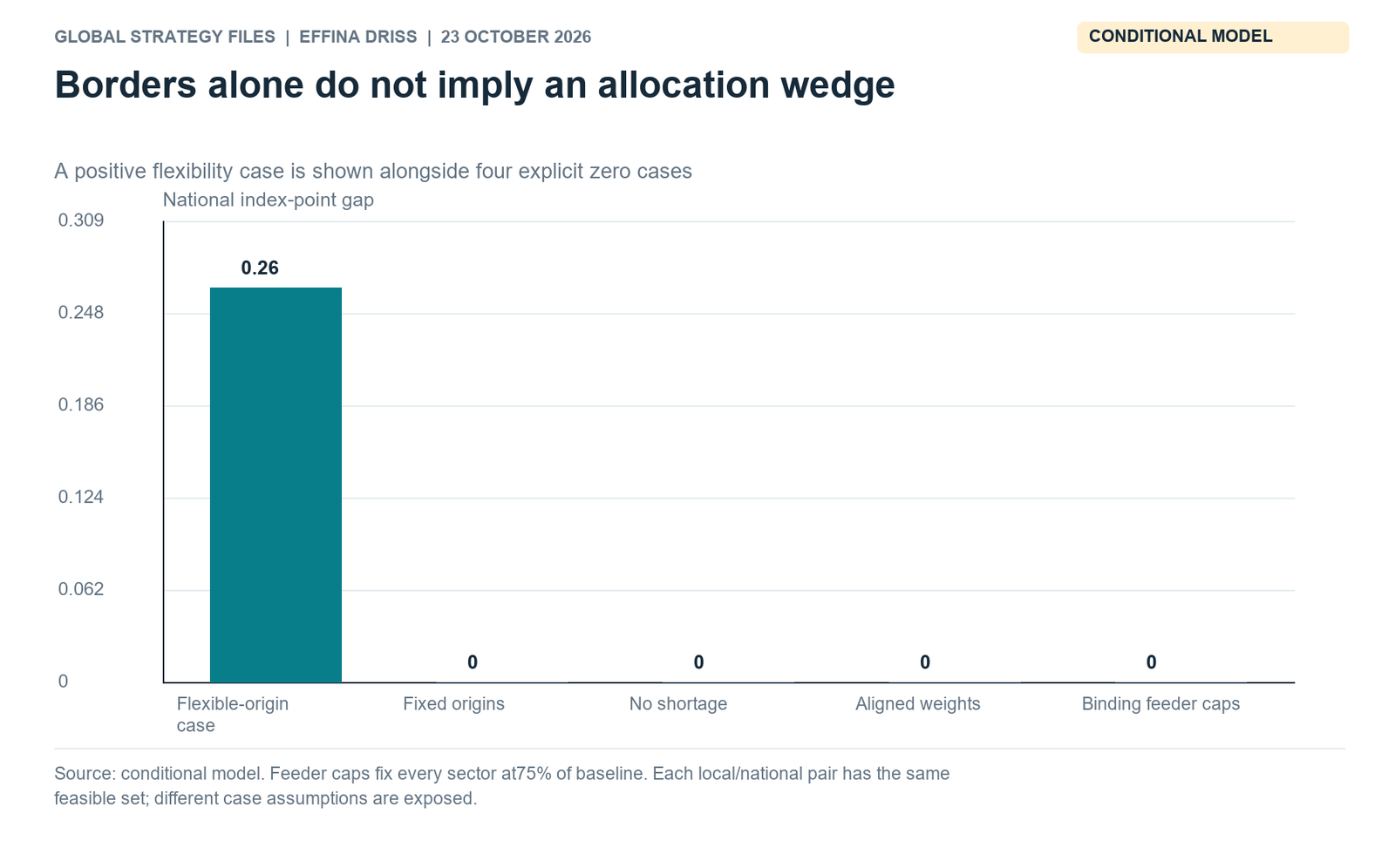
Figure 14 places the selected positive flexibility case beside four explicit zeros: fixed origins, no shortage, aligned objectives and binding common feeder caps. The cases change specified assumptions, while each national-local pair retains an identical feasible set. These zeros are central results, not robustness footnotes added after a favorable example. They reject a claim that the existence of fiscal borders or historical outside customers necessarily creates an additional national allocation loss under every shortage configuration.
With no shortage and baseline output caps, the historical allocation attains every positive output ceiling, so the model has no profitable reallocation margin. With aligned objective weights, the local endpoint counts the same value as the national objective, and any border label is irrelevant to this comparison. Neither zero proves that real administration is efficient: both follow from precise, deliberately simplifying conditions. Their purpose is to identify which additional facts a positive fiscal-border argument would have to establish.
The feeder case places a common 75% output cap on every sector. The proportional allocation of 75% of historical output, intermediate shipments and terminal deliveries is feasible and attains those caps. Under the published objective convention both endpoints deliver national index 75, and the fiscal gap is zero. This is a case where physical restrictions eliminate discretionary substitution even though the objective weights differ. It shows why observing a plant restriction does not establish that the authority could have chosen a better national allocation within the actual engineering constraints.
National policy supplies an additional institutional challenge. The November 2021 SME guidance calls for protection of key supply-chain enterprises, including upstream and downstream SMEs identified through leading firms. Such priorities can already incorporate value beyond a supplier’s own local tax contribution. A causal study must test their application instead of assuming all local authorities ignore network value. Taken together, the model zeros and this policy alternative make the positive mechanism conditional on both feasible choice and an actual divergence in priorities. (State Council: 2021 No.45 support for SMEs)
Continue reading
Get the complete 30-page research note
The English PDF includes 15 figures and 13 tables, the verified 2017 network, Wuyi priority arithmetic, 71 audited conditional programs, the complete non-monotone parameter grid and an explicitly assumed analytical appendix.
29 USD, instant PDF download, secure card payment.
Buy the full noteOne-time PDF-only purchase. Cutoff: 23 October 2026. No executed fiscal intent, national budget deficit or current GDP loss is estimated.
Need this analysis for your organisation?
We prepare confidential briefings, executive talks and studies on countries, markets and policies, built on the same method as this article.
Request a briefingSupport independent analysis
Our studies are free to read and carry no advertising. If this one was useful, a small contribution helps us publish the next.
Support our workGo further: books by Global Strategy Files

Books from Global Strategy Files
Go further on this topic
The Tariff GambleHow America’s trade war is reshaping power, prices and prosperity.24.99 USD, see the book Future-Proofing AmericaEconomic challenges and the road to reform.20 USD, see the book
 Kill KennedyWhat the 2025 declassified files reveal about the machinery of American power.20 USD, see the book