
China Export Invoices and Household Paydays

Driss EFFINA, PhD Independent Researcher, Global Strategy Files Decoded, China series, 24 October 2026.
Public accounts do not identify the chain from accepted export collection to worker receipt and purchases. This preview separates those records, then declares the complete employer budget, household preferences, information and terminal constraints before presenting conditional calendar results.
The missing evidence is a linked sequence of cash dates
The public records in this pilot do not establish that delayed accepted export invoices move Chinese workers’ wage credits or household purchases. They establish why commonly used receivable ratios, annual wage averages and employee-benefit liabilities cannot measure that chain. Invoice acceptance, contractual maturity, customer payment, employer cash availability, payroll transfer and employee receipt are different events. The original quantitative work therefore takes the form of an exposed daily accounting experiment and certified spending-plan bounds. Missing causal identification is the lead; it is not an estimate that no household ever experiences the proposed mechanism.
The evidence combines industrial release vintages covering 2015-2025, a separate actual January-August 2026 observation, wage releases and comparators covering 2014-2025, payment-record rules and Haier’s global consolidated accounts. These sources offer useful scale, classifications and warnings. They do not join a foreign buyer’s accepted invoice to the Chinese employing entity, a genuinely usable credit facility, a worker’s net payment and a dated household ledger. Haier’s disclosed employee-benefit payable is not evidence of overdue wages. The article makes no allegation of actual arrears at that issuer. (2026 Jan-Aug industrial accounts) (2025 annual wages) (Haier Smart Home Annual Report2025)
The conditional model asks a narrower question: with current jobs, agreed take-home principal and accepted invoice values fixed, when does a collection date cross a payroll deadline, and which resources absorb the timing change? The employer can use free cash, drawable credit or eligible factoring. A household can preserve spending with its own liquid assets even when wages arrive later. Those are distinct buffers at distinct accounts. Payment-processing delay supplies another route to late bank credit without employer transfer delay. The model’s counterexamples are part of its answer, rather than exceptions concealed after an adverse result.
Long-run receivable stocks provide context with a break
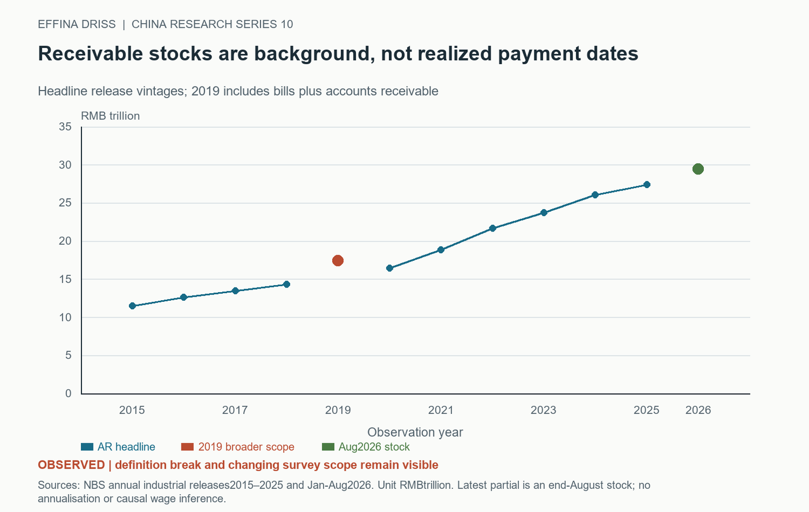
NBS industrial releases place accounts receivable at RMB 11.45469 trillion at end 2015, 16.41 trillion at end 2020 and 27.43 trillion at end 2025. Figure 2 retains the annual release-vintage observations and a separately labeled end-August 2026 stock of 29.48 trillion. The latest actual release also reports 7.36 trillion of finished-goods inventories. A stock can be observed at a partial-year date without becoming a full-year outcome or a forecast. These aggregates concern the published industrial survey, not only exporters or already accepted foreign invoices. (2015 industrial accounts) (2020 industrial accounts) (2025 industrial accounts) (2026 Jan-Aug industrial accounts)
The 2019 observation is explicitly broader: RMB 17.40 trillion of bills plus accounts receivable, rather than the AR-only headline used for surrounding years. Treating it as an ordinary point in an unchanged AR series would manufacture a level comparison. Earlier releases also use main-business revenue where later accounts use operating revenue. Survey coverage, comparators and release definitions can change. The original table preserves each source and definition; it does not infer a repayment-duration trend, a fixed-firm growth coefficient or a policy effect from endpoint differences. (2019 industrial accounts)
Benefit expense and payable balances are different accounts
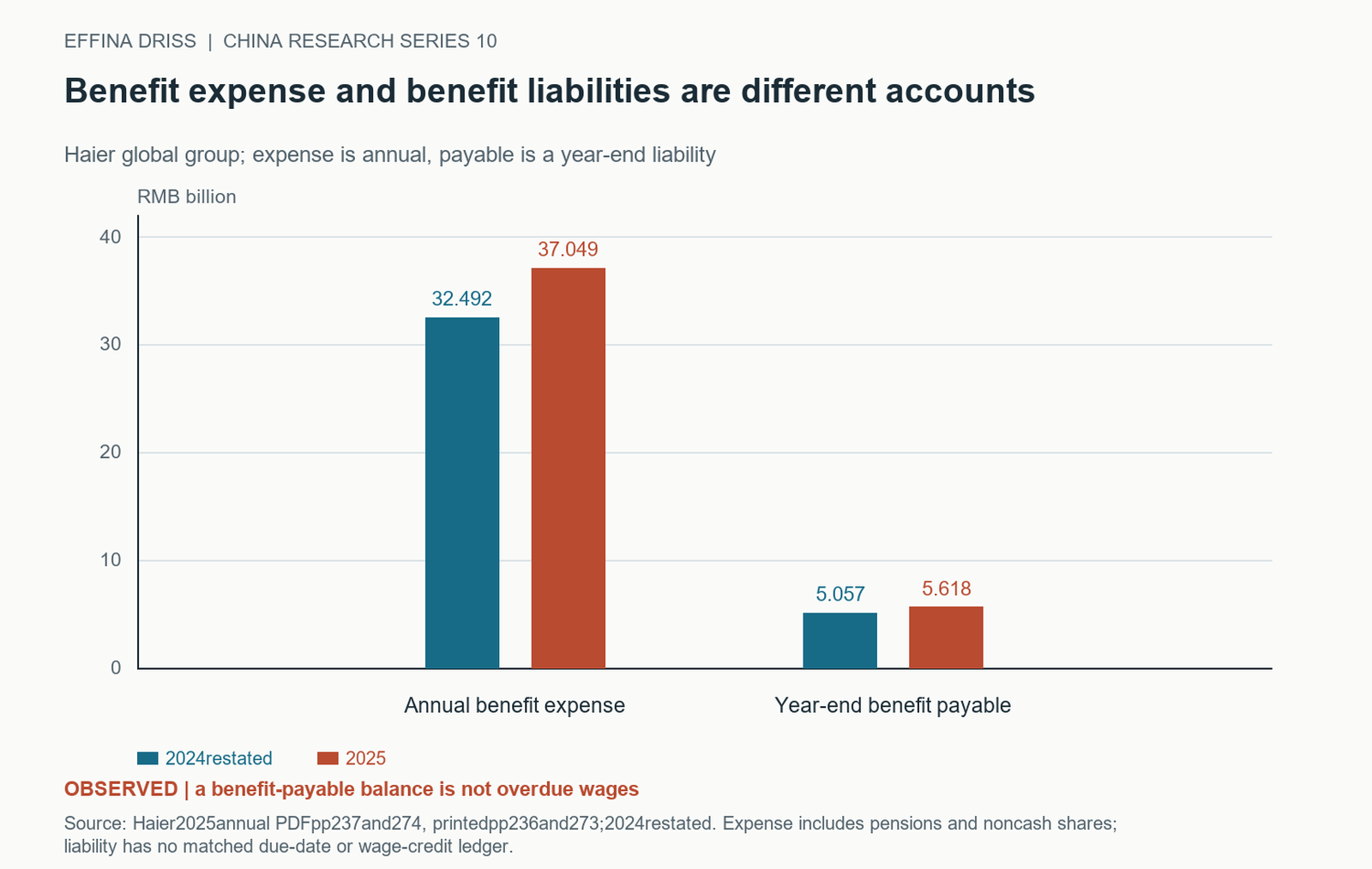
The same global report gives RMB 37,049 million employee-benefit expense in 2025, compared with a restated 32,492 million. The expense includes salaries, bonuses, allowances and benefits in kind of 33,791 million, pension expense of 2,768 million and equity-settled share expense of 490 million. Figure 6 keeps expense separate from the employee-benefit payable of 5,618 million, against 5,057 million in the restated comparator. They are different accounting objects and periods of measurement. (Haier Smart Home Annual Report2025)
A payable can represent a normally accrued amount not yet due. The note does not turn that balance into overdue take-home wages, and annual expense does not identify a worker’s bank-credit date. Noncash shares, pensions, deduction accounts, opening liabilities, acquisitions and classifications also matter before translating an accrual into paid cash. Subtracting the change in one aggregate payable from total benefit expense would not recover net employee bank credits without a complete adjustment ledger. No such payroll reconciliation was obtained. (Haier Smart Home Annual Report2025)
The distinction is central to the claim under study. It is possible to observe stable employment, a growing annual benefit expense and unchanged wage principal while the calendar of cash receipt differs. It is also possible to observe a payable with no late payment at all. The issuer accounts alone cannot select between those cases. The article uses them to prevent a false arrears measure and to specify the missing data. Actual due dates, amounts, deductions and receipt evidence are required before classifying a wage payment; the subsequent late-payment states are hypothetical stress experiments.
Declare the employer and household experiment before results
The calendar has 120 days and 100 equally paid workers. Each receives agreed net monthly pay of RMB 6,000; the employer owes 600,000 on days 15, 45, 75 and 105. Four already accepted invoices each have face 600,000 and normal collection on days 10, 40, 70 and 100. Only the first is delayed twenty days in the central comparison. Current jobs, wage principal, invoice face and exchange rate stay fixed. Other cash of 275,000 arrives on days 0, 30, 60 and 90; nonpay obligations of 200,000 fall on 12, 42, 72 and 102. A prior wage obligation of 50,000 is paid on day zero.
Initial free employer cash, credit and factoring are zero centrally. Named alternatives use free cash of 575,000, or a nominal 600,000 line with usable fraction one versus zero. Default credit access is day 10; late access is day 35. Interest is 12% annually on previous-day principal. Full factoring eligibility permits the entire first invoice and funds on day 12, two days after missed collection, at a 1.5% face fee; 0.3% of face is separately assumed real service use. Bank-credit lag is zero centrally and three days in a processing-only case with no collection shock. Another alternative reduces other receipts by 200,000 on day 30. All current wages and loans are paid by horizon end. Prompt payment precedes financing-cost minimization; no buffer opportunity cost is optimized. None is Haier calibration.
Each hypothetical household starts with RMB 3,000 plus an extra buffer of 0, 1,000, 3,000 or 6,000, with no population weights or household credit. Reference nondurables are 150 daily and rent 1,500 falls on days 20, 50, 80 and 110. Consumption before day 10 is fixed; afterward the household knows the conditional path. Twelve concave utility segments, each 25 per day, and a rent-delay penalty of 0.01 determine timing. Terminal cash must equal initial cash and rent must be cleared, imposing nondurables of 18,000 and rent of 6,000 over the horizon. This is a timing-only comparison, not evidence of unchanged actual annual consumption.
The decision objectives, cash identities and optimal-plan bounds below precede the numerical timing results. All dates are model days; holidays, payroll taxes, bankruptcy, household labor supply and endogenous order changes are omitted. Late-pay states are stress counterfactuals, not permission to delay lawful obligations. Table 6 fixes the complete dated normalization so that no later threshold can be mistaken for an estimated Chinese employer or household parameter.
Table 6. Complete dated normalization before numerical results
| Block | Assumed values | Constraint or scope |
|---|---|---|
| Employer calendar | 120 days; 100 workers; net 6,000 each; due 15/45/75/105 | Current wage principal fixed at 2.4 million |
| Receipts and obligations | Four invoices 600,000 at 10/40/70/100; other 275,000 at 0/30/60/90; nonpay 200,000 at 12/42/72/102; prior wages 50,000 at 0 | Only first collection moves 20 days centrally |
| Finance | B=0 central; usable fraction/access explicit; APR 12%; factor fee 1.5%, service 0.3%, funds day 12 if eligible | All loans and wages paid by horizon |
| Household resources | Initial 3,000 + extra 0/1,000/3,000/6,000; no household borrowing | No population weights |
| Preferences/information | 12 segments of 25 daily, slopes 1/sqrt(midpoint), max 300; rent 1,500 at 20/50/80/110; penalty 0.01; reveal day 10 | Before reveal, consumption 150/day |
| Terminal comparison | Cash equals initial; rent cleared | Nondurables 18,000 + rent 6,000 imposed |
Money RMB; days are model days. All inputs assumed, including perfect-information recourse. Timing-only resources do not establish unchanged actual annual consumption.
The objectives separate prompt payment from spending utility
Employer cash equals previous cash plus scheduled receipts, loan draws and net factor proceeds, less fixed obligations, current wage transfers, principal repayments and interest on previous-day debt. Loan principal equals its previous balance plus draws minus repayments and is bounded by genuinely accessible capacity. Cash stays nonnegative, wages cannot be prepaid before their cohort due date, and each cohort totals RMB 600,000 by the horizon. Terminal borrowing is zero. Later receipts make the delivered cases feasible; these constraints do not assert that every real employer can meet its obligations eventually.
The employer first minimizes wage amount-days after the agreed transfer date. It then minimizes private interest and factoring fees while preserving the first optimum within the declared tolerance. A coefficient of 1e-8 on gross draws and repayments discourages pointless financing round trips; it is a disclosed tie-breaker, not a resource cost. Employer LP money is internally in RMB thousand and reported outputs convert to RMB. The priority assumes prompt payment, rather than profit-maximizing wage withholding. Recourse knows the specified scenario path and estimates no actual employer preference.
The household chooses consumption and rent timing subject to nonnegative cash and unpaid rent. Its twelve consumption segments have decreasing slopes one divided by the square root of each segment midpoint, with a daily maximum of RMB 300. It maximizes consumption utility less 0.01 times rent amount-days unpaid. Utility units are not monetary damages. Before day 10 consumption remains 150; later decisions have perfect knowledge of the conditional path. Terminal assets and rent clearance enforce the fixed total resources stated on the setup above, while allowing catch-up spending.
After obtaining household optimal utility, two more LPs minimize and maximize spending over days 15-29 while keeping the utility objective within 1e-7 of its optimum. That interval bounds equally optimal plans; it is neither a confidence interval nor a distribution across households. Daily curves show one optimum where ties remain. These identities and the optimization hierarchy precede the numerical model outcomes. No fitted behavioral coefficient, forecast distribution or observed Chinese asset frequency enters this calculation.
An on-time partial credit can conceal a late completion
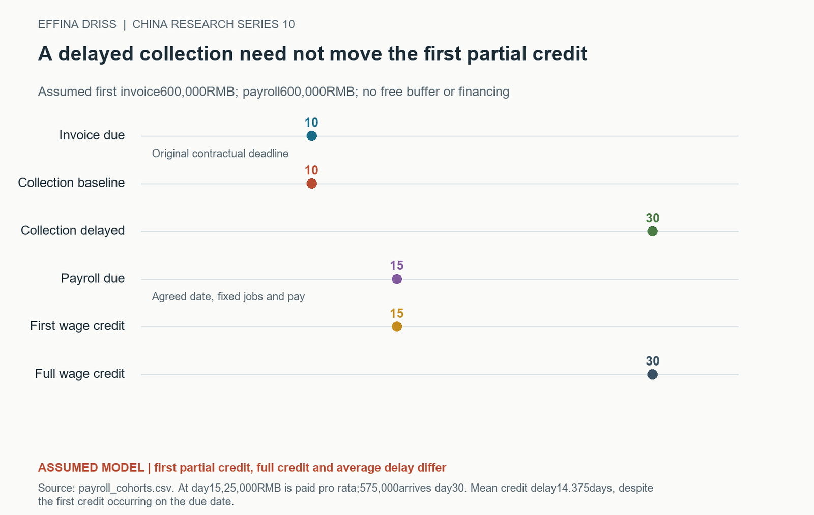
With the first collection shifted from day 10 to day 30, the employer has RMB 25,000 available at payroll day 15 after the stipulated other cash, nonpay obligation and prior wage. It transfers that amount and completes the remaining 575,000 on day 30. Under equal pro-rata allocation each of the 100 workers receives 250 on the agreed day and 5,750 fifteen days later. Figure 7 therefore separates an on-time first partial credit from full-credit lateness. Neither date alone is a sufficient summary of the wage event.
The first cohort’s amount-weighted delay is 14.375 days, obtained from 575,000 times fifteen divided by 600,000. Its transfer-delay area is 8.625 million RMB-days. This is a timing exposure, not RMB 8.625 million of wage loss or a national worker estimate. Default bank lag is zero here, so employer transfers and worker credits coincide. Later payrolls are on time to the displayed tolerance and all current wage principal still totals 2.4 million across the horizon. The central episode closes before the second payroll is due.
An empirical file that calls the cohort paid because a first deposit arrived would miss most of this timing change. A file that treats all 600,000 as fifteen days late would overstate the amount-days area by ignoring the partial payment. The constructed example demonstrates the value of retaining every amount and date; it does not claim employers use equal partial allocations in reality. Actual payroll batching, worker priority, deductions and cash payments would require their own records before applying this accounting summary to a firm.
An optimal-plan interval is not a confidence interval
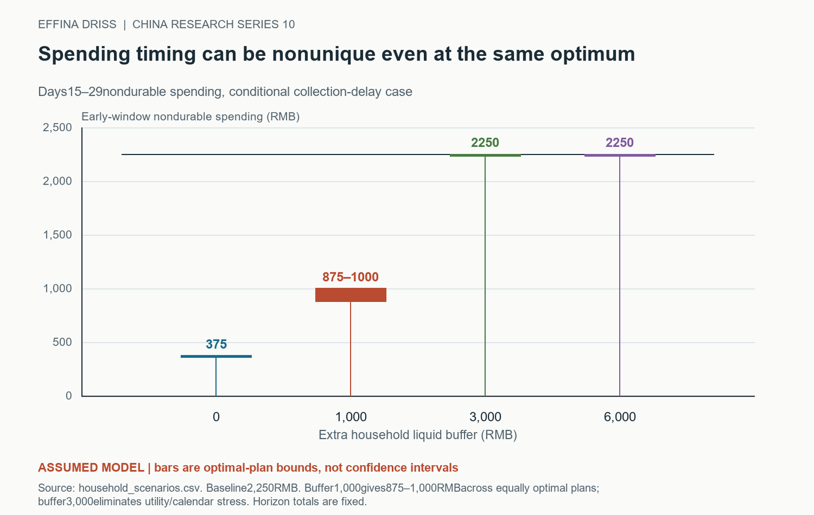
For days 15-29, baseline nondurable spending is RMB 2,250. Under the central delayed wage path and no extra household buffer, optimal spending in that window is 375, to numerical tolerance. The difference is 1,875 for this hypothetical household and interval. It is not a loss of wage principal, a national consumption estimate or an annual spending effect. Later catch-up is permitted and total horizon nondurables are fixed by the resource and terminal constraints.
With RMB 1,000 extra liquidity, the minimum and maximum early spending compatible with optimal utility are 875 and 1,000. Figure 12 gives that range priority over a single selected daily plan. The interval reflects multiple solutions to the same assumed optimization problem at its declared tolerance. It is not a confidence interval, an empirical treatment-effect bound or the distribution of spending across a thousand observed workers. The model supplies no population probabilities for the buffer categories.
At extra buffers of 3,000 and 6,000, the optimal early-window amount returns to 2,250 with baseline utility. This provides a direct disconfirmation of a necessary purchase response to late wages. The low-buffer stress depends on rent dates, available cash, concavity, the maximum daily consumption segments, information and terminal conditions. Changing any of those assumptions can change both the interval and its interpretation. Their exposure makes the result reproducible; it does not validate them as household behavior. The empirical task remains to observe resources and purchases in a linked sample.
Continue reading
Get the complete 30-page research note
The English PDF contains 15 scientific figures, 11 tables, long-run source/vintage checks, a global issuer scope audit and a certified daily employer-household model with explicit thresholds, spending-plan bounds and zero cases.
29 USD, instant PDF download, secure card payment.
Buy the full noteOne-time PDF-only purchase. Evidence cutoff: 24 October 2026. Missing linkage is not a zero causal estimate. Household horizon totals are imposed for a timing-only comparison. No actual issuer arrears or national consumption loss is alleged.
Need this analysis for your organisation?
We prepare confidential briefings, executive talks and studies on countries, markets and policies, built on the same method as this article.
Request a briefingSupport independent analysis
Our studies are free to read and carry no advertising. If this one was useful, a small contribution helps us publish the next.
Support our workGo further: books by Global Strategy Files

Books from Global Strategy Files
Go further on this topic
The Tariff GambleHow America’s trade war is reshaping power, prices and prosperity.24.99 USD, see the book Future-Proofing AmericaEconomic challenges and the road to reform.20 USD, see the book
 Kill KennedyWhat the 2025 declassified files reveal about the machinery of American power.20 USD, see the book