China Electric Vehicles and Road Finance


Driss EFFINA, PhD Independent Researcher, Global Strategy Files Decoded, China series, 24 October 2026.
Equal replacement changes the starting question
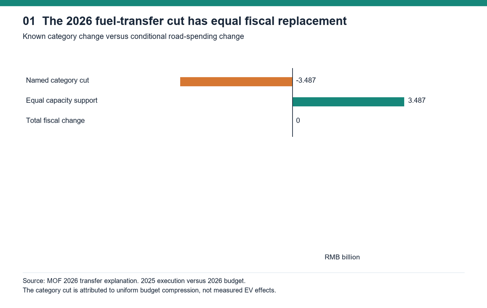
China’s 2026 budget reduces a named fuel-reform transfer by RMB3.487 billion while providing planned equal financial-capacity support to the affected provinces. That is a change in budget categories, not an observed EV-caused loss of local road resources. The road component depends on how both categories are spent: it is exactly zero when their road-directed shares are equal. A separate maintenance grant falls from RMB19.801 billion in 2025 execution to a 2026 budget of RMB18.811 billion, with substantial redistribution across its nonduplicated recipients. These observations motivate an original, fully assumed allocation model. In that experiment, restoring aggregate resources does not necessarily restore every regional service floor; allocation caps, industrial-gain geography and uncertain commitments matter. Alignment provides an explicit counterexample. The analysis identifies accounting conditions and certified conditional bounds, while actual province-level net EV effects remain unidentified.
The Ministry of Finance attributes the category reduction to uniform budget compression. Its explanation states that the compressed resources increase financial-capacity support and return in equal amounts to the provinces whose categories were cut. Neither the stated cause nor the replacement can be omitted from an analysis of the transition away from liquid fuels. The verified result concerns a 2026 budget policy; the package does not observe its full-year execution or the eventual road-spending choices of every recipient. (2026 central to local transfer budget explanation)
This distinction changes the empirical task. Falling fuel consumption can threaten a revenue base, but a province’s road resources also depend on pooled transfers, other grants, own charges, industrial fiscal resources and expenditure commitments. The location of vehicle production, fuel purchase or registration is not automatically the location retaining the associated tax. The article therefore starts with the actual fiscal institutions and public accounts, then asks what an explicit allocation experiment can establish.
Central pooling separates tax location from road responsibility
The Ministry of Finance’s 2018 reply identifies refined-oil consumption tax and reform-related ancillary revenue as central revenue. Apart from central replacement expenditure, reform receipts support transfers to local governments. The reply distinguishes the place of collection from the consumer bearing the burden: allocating ancillary receipts to refinery locations would shift resources away from other regions. A map of refineries or petrol purchases is consequently not a map of local road money. This institutional observation is essential before relating electrification to a provincial budget. (Fuel tax reform follow-up reply fiscal letter 2018-150)
The road component is zero when spending shares match
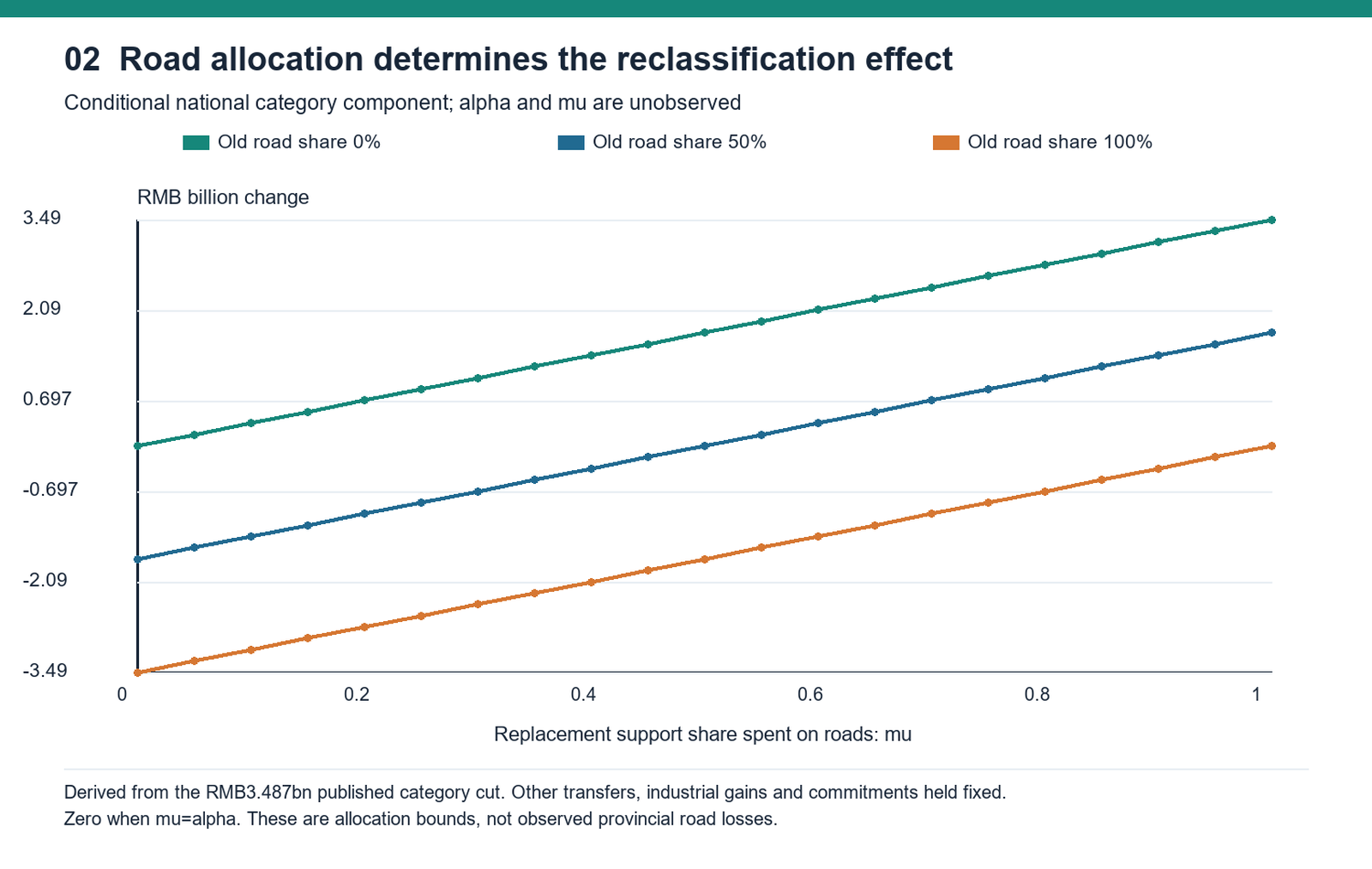
Let d be a positive category reduction, alpha the share of the old category directed to roads and mu the corresponding share of replacement financial-capacity support. Hold other resources and commitments fixed. The isolated road-resource change is d(mu-alpha). This expression counts the category reduction and replacement once each, rather than treating the former as a loss and ignoring the latter. For the published national d of RMB3.487 billion, equal shares give exactly zero.
If the old category directs 80% to roads and replacement support directs 60%, the component is minus RMB0.6974 billion. Reversing those shares makes the component plus RMB0.6974 billion. These are arithmetic examples, not observed Chinese spending shares. The source does not establish that every yuan of the old category financed road maintenance, and unrestricted financial support is not automatically spent entirely on roads. Naming both shares makes the missing evidence visible. (2026 central to local transfer budget explanation)
With alpha and mu each limited only to the interval zero to one, the component lies between minus RMB3.487 billion and plus RMB3.487 billion. A one-sided range from minus RMB3.487 billion to zero adds the assumption that alpha equals one. Neither interval is a confidence interval. Figure 2 holds the other fiscal channels fixed; it does not assign the endpoint to a province or estimate how road-spending preferences respond to electrification.
The equality case is a substantive disconfirmation of an automatic-loss claim. It does not prove every province keeps the same road allocation. It identifies precisely what must be measured to move from a known category change to a road-resource result: the relevant old and replacement spending shares, actual execution and their consolidation with other accounts.
The observed maintenance account does not show a collapse
National general-public-budget final accounts report highway-maintenance expenditure of RMB88.583 billion in 2020, 116.967 billion in 2022, 123.146 billion in 2023, 124.227 billion in 2024 and 136.266 billion in 2025. These are actual national expenditure classifications, rather than central-level-only amounts. The missing 2021 value is left missing. The five observations should not be mistaken for a complete historical panel or all economic costs of preserving the network. (2020 national general public budget expenditure final accounts) (2022 national general public budget expenditure final accounts) (2023 national general public budget expenditure final accounts) (2024 national general public budget expenditure final accounts) (2025 national general public budget expenditure final accounts)
Dividing by same-year total highway route length gives approximately RMB17,041, 21,843, 22,650, 22,626 and 24,425 per route kilometer, respectively. The nominal ratio rises over this selected window, with a small decline in 2024. That observation contradicts a claim that this particular national account has already demonstrated a general collapse per broad route kilometer. It does not establish adequate maintenance, a real-price improvement or the absence of local pressure.
A separate maintenance grant requires a separate ledger
The original Ministry of Finance regional-transfer PDF provides a maintenance-related grant following cancellation of government-loan secondary-road tolls. Its printed page 66 gives 2025 budget, 2025 execution and 2026 budget; page 67 explains scope and performance. Following repayment of relevant cancellation debts, the fund supports ordinary national/provincial and rural non-toll road maintenance. Road length, maintenance performance and fiscal difficulty are among the allocation considerations. This is a separate program from the fuel-reform transfer discussed earlier. (2026 regional transfer tables)
The printed national amounts are 200.00, 198.01 and 188.11 hundred million RMB, or RMB20.000, 19.801 and 18.811 billion. Comparing the 2026 budget with 2025 execution gives a reduction of RMB0.990 billion; comparing budgets gives RMB1.189 billion. The baseline changes the arithmetic. Neither figure is the RMB3.487 billion fuel-category reduction, and neither is an estimate of a national road-financing gap caused by EVs.
All 43 printed rows are retained. For arithmetic totals, a distinct table uses the 31 provincial-level units plus XPCC, giving 32 recipients. Inclusive provincial rows are not added to separately displayed subcities or province-excluding-subcity rows. Summing rounded top-level amounts differs from the printed national totals by plus 0.01, plus 0.01 and minus 0.01 hundred million RMB in the three columns. These small residuals stay visible; no balancing jurisdiction is invented.
Table 3. The maintenance grant is distinct from fuel-reform transfers
| Measure | Amount or count | Status |
|---|---|---|
| 2025 grant budget | RMB 20.000 billion | Plan |
| 2025 grant execution | RMB 19.801 billion | Reported actual |
| 2026 grant budget | RMB 18.811 billion | Plan |
| 2026 minus 2025 execution | Minus RMB 0.990 billion | Derived change |
| Recipients / printed rows | 32 / 43 | Deduplicated / full transcription |
| Rounding residuals | +1 m / +1 m / -1 m RMB | Top-level sums minus totals |
Original MOF PDF printed pages 66-67. Thirty-one provinces plus XPCC; inclusive provinces and separately shown subcities are not added. (2026 regional transfer tables)
The synthetic economy is fully normalized before results
Set the starting transferable pool to one normalized fund unit. It is not one yuan, one percent of GDP or the observed fuel-reform budget. There are three unnamed archetypes: road-heavy, producer and mixed. Fixed bases are [0.35, 0.20, 0.15], residual-growth weights [0.50, 0.20, 0.30], and road-service shares [0.60, 0.10, 0.30]. Their values are assumptions. The institutional sources motivate examining separate bases and growth, but do not supply these numbers. (Fuel reform transfer reply fiscal letter 2022-23)
The bases total 0.70, leaving a starting growth component of 0.30. Initial transfers are consequently [0.50, 0.26, 0.24]. Dividing by the service shares gives starting rates of approximately 0.833333, 2.600000 and 0.800000, so the initial common minimum is 0.80. The producer archetype’s high rate follows from its small assumed service share; it is not a statement about any Chinese manufacturing province.
A shock delta contracts the pool, and optional buffer b gives available resources P=1-delta+b. The central reported comparison uses delta=0.25, with additional compensation C kept distinct from the residual pool. Retained road-directed industrial gain is G=0.12, distributed by a specified geography. Additional commitments are separately introduced in the robust case. No EV share is mapped into delta, G, service or costs, and no coefficient is fitted to the descriptive series.
This setup permits transparent policy comparisons. Pool, gains and service are held fixed when grants are reallocated; a grant is not counted as both compensation and new industrial money. The objective will be the lowest resource/service rate across regions and declared scenarios. This is an explicit fairness criterion, not an estimated utility or welfare function. Readers who prefer a different criterion can alter the exposed program rather than mistake the chosen objective for an observed policy law.
Normalization is homogeneous: multiplying every resource, base, gain, compensation and cap by the same positive factor multiplies the reported monetary levels without changing the allocation logic. It does not provide permission to choose that factor from an unrelated public budget. A substantive RMB calibration needs measured coverage and parameters for the actual recipients. The model remains informative at unit scale because its targets and feasibility restrictions can be derived exactly.
Complete the model setup before interpreting its thresholds. At pool P=1-delta, bases have priority while P is at least 0.70: transfers equal bases plus growth weights times (P-0.70). Below that boundary, bases are rationed proportionally. The point industrial-gain shares are [0.10,0.70,0.20], with no additional point costs. The robust set has four gain-share vertices: [0,0.50,0.50], [0,0.80,0.20], [0.20,0.50,0.30] and [0.20,0.80,0]. Additional upper commitments are [0.02,0.03,0.02]. One nonnegative grant vector is chosen before the vertex is known, totals compensation C, and has nonbinding caps of 10 per recipient. It maximizes the lowest resources per service share. Existing industrial gains cannot be reassigned. Every numerical input is assumed; the robust set is not a confidence interval and the archetypes are not named provinces.
Restoring the national total need not restore local floors
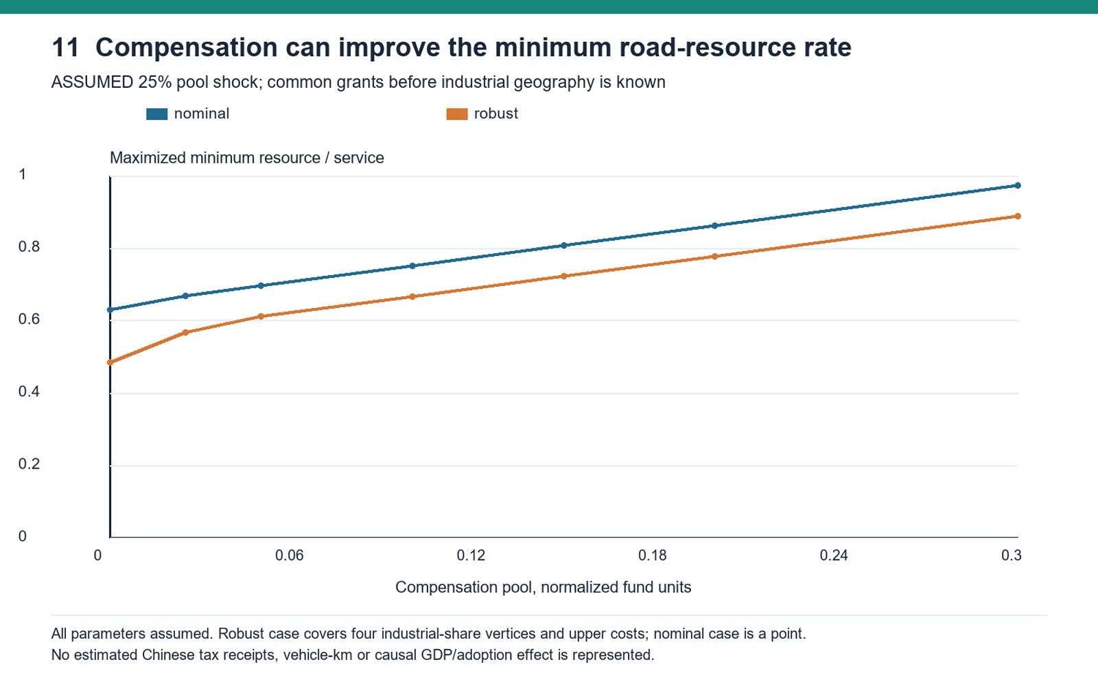
The point case starts with a 0.25 pool contraction and a 0.12 industrial gain, leaving aggregate pre-compensation resources of 0.87. Compensation of 0.13 restores the total to 1.00. Yet the best minimum rate is only 0.784444, below the initial common floor of 0.80. This is not a missing-resource paradox. The producer retains its concentrated gain, grants are nonnegative, and existing resources cannot be reassigned. More aggregate money can sit above the target in one region while another remains below it.
To restore the common 0.80 floor, each target is 0.80 times its service share. Against point resources [0.387,0.294,0.189], positive deficits are 0.093, 0 and 0.051, totaling 0.144. Restoring each region’s own initial transfer instead gives positive deficits 0.113, 0 and 0.051, totaling 0.164. The producer’s initial resource/service rate was above 0.80, so the common-floor and individual-restoration targets are not the same promise.
At every robust geography vertex, aggregate pre-compensation resources equal 0.80. Compensation of 0.20 restores each vertex’s total to one, while the common-grant worst-case floor is 0.777778. A single policy that guarantees the initial common floor needs 0.22; preserving every initial regional allocation under every vertex needs 0.26. These thresholds use componentwise worst-case regional resources and the nonnegative-grant constraint.
Table 7 separates the six thresholds so they cannot be combined into one asserted cost of electrification. They are normalized, assumed-policy bounds. Permitting reassignment of existing industrial gains, choosing grants after uncertainty resolves, changing service responsibility or relaxing a target alters the feasible set. The result establishes why a compensation promise should state what is preserved: aggregate capacity, a common service floor or each region’s earlier allocation.
These thresholds are lower bounds attained when the default recipient caps are nonbinding and funds can be assigned wherever a positive deficit remains. They do not include administrative implementation costs or endogenous changes in service. A cap below a required regional deficit can make the target infeasible regardless of additional compensation elsewhere. Reporting a restoration amount without those feasibility conditions would turn a conditional mathematical result into an unsupported funding promise.
Alignment removes the allocation wedge entirely
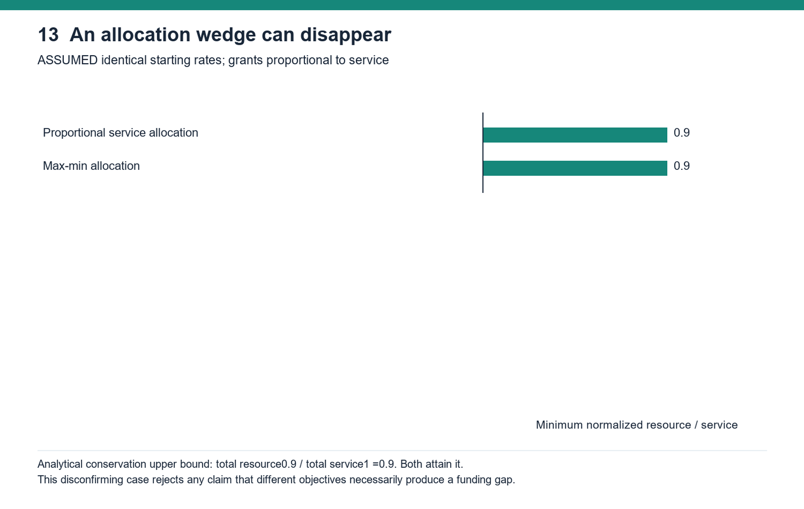
The aligned case begins with regional resources equal to 0.80 times service shares. Initial rates are therefore identical. Compensation of 0.10 is then allocated in proportion to service, giving 0.10 times service shares. Every region reaches 0.90. The max-min optimizer reaches the same 0.90, with zero difference. No region can have a minimum above the aggregate resource/service ratio of 0.90 when total service is one.
This is an exact conservation argument, not a favorable selection from noisy simulations. It shows that different allocation approaches do not necessarily produce a wedge. The earlier advantage of floor-oriented grants depends on initial imbalances, the gain geography, commitment treatment and constraints. If those conditions align resources with service, a simple proportional rule already attains the chosen objective.
The conditional alpha=mu accounting identity provides a separate zero. Matching road-directed shares makes the isolated 2026 category reclassification road-neutral even when budget labels change. The alignment scenario instead concerns how a fully assumed compensation pool is distributed across service responsibilities. Their mechanisms differ, so observing one would not automatically establish the other. Together they prevent a narrative in which every fiscal rearrangement inevitably worsens regional road funding.
A policy claim should survive these counterexamples by stating its conditions. A useful claim is that concentrated gains and constrained new grants can make aggregate replacement insufficient for a local floor. An unsupported claim is that EV adoption must create a road-finance deficit wherever production and road use differ. The original experiment strengthens the former by making the latter’s failure explicit. Figure 13 keeps the zero case visible beside the larger conditional gaps.
Continue reading
Get the complete 30-page research note
The English PDF includes 14 scientific figures, 10 tables, primary-source account reconstruction, exact allocation bounds, explicit model assumptions and disconfirming cases.
29 USD, instant PDF download, secure card payment.
Buy the full noteOne-time purchase. Evidence cutoff: 24 October 2026. Conditional allocation results are not measured provincial EV losses.
Need this analysis for your organisation?
We prepare confidential briefings, executive talks and studies on countries, markets and policies, built on the same method as this article.
Request a briefingSupport independent analysis
Our studies are free to read and carry no advertising. If this one was useful, a small contribution helps us publish the next.
Support our workGo further: books by Global Strategy Files

Books from Global Strategy Files
Go further on this topic
The Tariff GambleHow America’s trade war is reshaping power, prices and prosperity.24.99 USD, see the book Future-Proofing AmericaEconomic challenges and the road to reform.20 USD, see the book
 Kill KennedyWhat the 2025 declassified files reveal about the machinery of American power.20 USD, see the book