The Last Budget Before the Vote: Italy’s Escape Clause and the Electoral Fiscal Cycle


Executive Summary
On 13 October 2026 the Italian government sent Brussels its draft budgetary plan for 2027, the last full budget before the general election due in the second half of next year. The plan is a package of about 23.5 to 26 billion euros. It cuts taxes for middle-income families, raises spending on families, health and public wages, funds energy relief for households and firms, and increases defence outlays. Roughly 5 billion euros comes from higher taxes on banks, insurers and energy companies, and further amounts from spending cuts across ministries and from gaming. The rest is borrowed. The headline deficit, which the government expects to fall to 2.9 per cent of GDP in 2026, is planned to rise to 3.4 per cent in 2027 and 3.3 per cent in 2028.
The legal vehicle for this borrowing is the national escape clause, a provision of the reformed European fiscal rules that lets member states spend more on defence, and in the 2026 version on energy security, without breaching their agreed expenditure paths. The Commission recommended on 8 October that the Council allow Italy to use it, and the Ecofin Council takes up the request on 9 November. Italy asks for room worth 0.6 per cent of GDP in each of 2027 and 2028, about 14 billion euros a year. Net of that allowance, the government argues, the deficit is 2.8 per cent in 2027 and below 3 per cent throughout, which would let Italy leave the excessive deficit procedure next year.
This paper looks past the legal question to the economic one. Does the 2027 budget follow a pattern, and what will the extra borrowing buy? It builds a panel of thirteen EU countries over 1995 to 2025 with about 100 general elections, estimates the electoral fiscal cycle and ranks countries by its strength. It then estimates Italian fiscal multipliers with a structural vector autoregression on quarterly data from 1999 to the second quarter of 2026, tests them across samples and specifications, and applies them to the composition of the 2027 package. Finally it traces the debt and interest legacy of the escape clause over ten years. Five findings stand out.
- Italy has the strongest electoral fiscal cycle in the sample. Across thirteen EU countries, primary balances deteriorate by about 0.2 to 0.4 points of GDP in election and pre-election years, an effect that is real but statistically imprecise. In Italy the gap is 0.88 points: in election and pre-election years the primary balance moves 0.88 points of GDP worse than in other years, after removing the common European fiscal stance, the business cycle and mean reversion. That is the largest of the thirteen countries, ahead of Ireland and France, and the only one where the gap approaches one point.
- The 2027 budget is an almost exact replica of the historical pattern. The panel model predicts that a country with Italy's characteristics, in an election year with growth of 0.8 per cent, will loosen its primary balance by 0.48 points of GDP. The government's own plan moves the primary surplus from about 1.0 per cent of GDP in 2026 to 0.5 per cent in 2027: a loosening of 0.5 points. What is new is not the size of the loosening but its packaging. In 2026, the year before the election, Italy tightened to escape the excessive deficit procedure; the electoral loosening has been concentrated in a single year and channelled through a European clause.
- Italian fiscal multipliers are low, and they depend heavily on the type of spending. The structural VAR finds that a euro of government consumption, which in Italy is mostly public wages and purchases of goods and services, raises GDP by about 0.7 euros after two years, with a wide uncertainty band. A euro of tax increase lowers GDP by between 0.13 and 0.27 euros. A euro of total government spending, which includes transfers and subsidies, raises GDP by only about 0.04 to 0.06 euros. The more of the budget goes to transfers and bonuses, the less it moves output.
- The escape-clause money buys little growth. Applying these multipliers to the composition of the package, with an allowance for the high import content of defence equipment, the 14.4 billion euros of escape-clause spending in 2027 raises GDP by about 3.8 billion euros, or 0.15 per cent. Every euro of extra deficit buys about 26 cents of output, and only about 13 per cent of the cost comes back through higher tax revenue. The budget as a whole, after the tax increases on banks and the spending cuts that partly finance it, adds about 0.16 per cent to GDP in 2027. That is a fifth of the 0.8 per cent growth the government forecasts for the year.
- The debt legacy outlasts the election by a decade. Because the interest rate on new Italian debt now exceeds nominal growth, the 1.2 points of GDP borrowed in 2027 and 2028 do not fade away. They are still 1.27 points of GDP in 2036 and by then cost about 1.4 billion euros a year in interest. On standard estimates of how sovereign spreads respond to debt, the escape clause adds 2 to 5 basis points to the BTP-Bund spread on its own.
The central argument is that the escape clause has turned a familiar electoral loosening into a European-sanctioned one, without changing its economics. The money will be spent mostly on transfers and imported equipment, where Italian multipliers are lowest, and paid for in a period when debt no longer erodes on its own. The clause solves a legal problem for Rome and a political problem for Brussels. It does not solve Italy's economic problem, which is that every point of borrowing now stays on the books.
1. A Budget With Two Deficits
Italian budgets are always negotiated twice: once in Rome and once in Brussels. The 2027 budget is unusual because it arrives in Brussels with two deficit figures. The headline figure, the one that Eurostat will eventually publish, is 3.4 per cent of GDP in 2027 and 3.3 per cent in 2028, above the 3 per cent reference value of the Treaty. The second figure is the deficit net of the national escape clause: 2.8 per cent in 2027 and 2.7 per cent in 2028. On the government's reading, the second figure is the one that matters for the excessive deficit procedure, because spending covered by the clause is, by construction, outside the rules (Figure 1).

The figure tells a story of a long road back. Italy ran deficits close to 3 per cent through the 2010s, saw them balloon to 9.4 per cent of GDP in 2020 and stay above 7 per cent through 2023 as the Superbonus tax credits for home renovation were recorded, then brought them down to 3.4 per cent in 2024 and 3.1 per cent in 2025. In September 2026 Istat confirmed the 2025 deficit at 3.1 per cent, just above the threshold, which kept Italy in the excessive deficit procedure for another year. The government expects 2.9 per cent in 2026. If that is confirmed in the spring of 2027, Italy will have satisfied the condition for leaving the procedure.
Then the line goes up again. The escape clause adds 0.6 points of GDP to the deficit in each of 2027 and 2028. The clause was designed in 2025 to let member states raise defence spending after Russia's war in Ukraine and the new NATO commitments. In 2026, as the conflict in the Gulf drove European gas and electricity prices to their highest levels since 2022, the Commission extended its use to measures for energy security. Italy requested activation in the summer, Parliament voted the authorisation, and the government has written the clause into its medium-term plan. The draft budget splits the allowance roughly equally between energy relief and defence.
There is nothing illegal or even unusual in this. Several member states have activated the clause, some of them, like Germany, on a far larger scale. The questions this paper asks are different. Is the timing a coincidence? Would Italy have loosened in 2027 anyway? And, because the clause relaxes the rules but not the arithmetic of debt, what does the extra borrowing buy, and what does it cost?
1.1 The package in numbers
The detailed content of the budget law is still being amended in Parliament, but the draft budgetary plan and the government's own statements allow a stylised breakdown (Table 1). On the spending and tax-cut side there are four blocks: energy relief financed through the escape clause, defence spending financed through the escape clause, measures for families and a further cut in personal income tax for middle incomes, and a set of other spending items including the renewal of public-sector contracts, health and investment. On the financing side there are three: higher taxes on the financial sector, including an increase in the regional business tax rate for banks and insurers and a reduction in deductions; spending cuts across ministries; and other measures, mainly from gaming concessions and tax compliance.
Table 1. Stylised composition of the 2027 budget, EUR billion
| Block | 2027 | Financing |
|---|---|---|
| Energy relief for households, firms and public buildings | 7.2 | Escape clause (deficit) |
| Defence and security | 7.2 | Escape clause (deficit) |
| Families and income tax cut for middle incomes | 5.0 | Ordinary resources |
| Other spending (public wages, health, investment) | 5.0 | Ordinary resources |
| Banks, insurers and energy companies | minus 5.0 | Tax increase |
| Ministry spending cuts | minus 3.5 | Expenditure review |
| Other covers (gaming, compliance) | minus 1.5 | Various |
| Net effect on the deficit | 14.4 | About 0.6% of GDP |
Note: Author's stylised breakdown based on the Documento programmatico di bilancio 2027 and government statements of October 2026. Gross size about 24 billion euros, within the 23.5 to 26 billion euros range reported. The escape-clause allowance of 0.6% of GDP corresponds to about 14 to 14.4 billion euros.
Two features of this composition matter for what follows. First, more than half of the gross package is financed by borrowing under the clause, and the ordinary part of the budget, the part that has to respect the expenditure path, is roughly neutral: about 10 billion euros of new measures against about 10 billion euros of covers. Second, the borrowed money goes to two kinds of spending that, as Section 4 shows, have unusually low effects on Italian output: transfers and price subsidies for energy, and defence procurement, much of which is imported.
1.2 Data and methods
The paper uses three sets of data (Table 2). For the electoral cycle it uses Eurostat's excessive deficit procedure notification data on the general government balance and interest payments for thirteen EU countries from 1995 to 2025, real GDP growth from the national accounts, and the dates of national legislative elections. For the multipliers it uses Eurostat's quarterly, seasonally and calendar adjusted, government finance statistics and quarterly national accounts for Italy from the first quarter of 1999 to the second quarter of 2026. For the budget it uses the government's draft budgetary plan and medium-term projections.
Table 2. Data used in this paper
| Series | Source | Span |
|---|---|---|
| General government balance and interest, % of GDP | Eurostat (gov_10dd_edpt1) | Annual, 1995 to 2025, 13 countries |
| Real GDP growth | Eurostat (nama_10_gdp) | Annual, 1996 to 2025 |
| National legislative elections | National electoral authorities | 1995 to 2025, about 100 elections |
| Total government expenditure and revenue, seasonally adjusted | Eurostat (gov_10q_ggnfa) | Quarterly, 1999 Q1 to 2026 Q2 |
| Real GDP, real government consumption, GDP deflator | Eurostat (namq_10_gdp) | Quarterly, 1999 Q1 to 2026 Q2 |
| Budget plan, deficit and debt projections | Documento programmatico di finanza pubblica and di bilancio 2027 | 2026 to 2029 |
Note: The thirteen countries are Austria, Belgium, Denmark, Finland, France, Germany, Ireland, Italy, the Netherlands, Poland, Portugal, Spain and Sweden. Greece is excluded because its fiscal series are dominated by the 2010 to 2018 adjustment programmes.
The methods are a fixed-effects panel regression of changes in the primary balance on election timing, an event study of fiscal behaviour around elections, a country-by-country index of the strength of the electoral cycle, a structural vector autoregression identified in the manner of Blanchard and Perotti (2002), bootstrap confidence bands and robustness checks, and a debt-dynamics simulation consistent with the second paper in this series.
2. Thirty Years of Elections and Budgets
The idea that governments spend more and tax less before elections is old. Nordhaus (1975) described a political business cycle in which incumbents engineer booms before the vote. Rogoff (1990) recast it as a signalling game: competent governments show their quality by delivering visible benefits before elections, at the cost of budget deficits. The empirical literature, surveyed by Brender and Drazen (2005) and many since, finds that electoral fiscal cycles are larger in new democracies and in countries with weak fiscal institutions, and smaller in established democracies with transparent budgets.
Italy is an established democracy with a long record of fiscal rules, from the Maastricht convergence effort of the 1990s to the balanced budget amendment of 2012 and the new European framework of 2024. One might expect its electoral cycle to be small. The data suggest otherwise.
2.1 The Italian record
Figure 2 shows Italy's primary balance, the budget balance excluding interest payments, from 1995 to 2025, with election years and the years before elections shaded, and the government's plan to 2029.
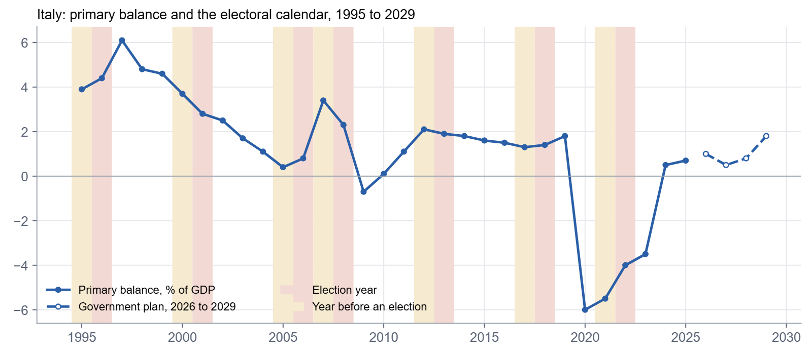
Several episodes stand out. The primary surplus peaked at 6.1 per cent of GDP in 1997, the year Italy qualified for the euro, and then fell in every year from 1998 to 2005. The decline was steepest around the elections of 2001 and 2006: the surplus fell by 0.9 points in both 2000 and 2001, and by 0.7 points in 2005, the year before the 2006 election, when it reached its lowest point of the pre-crisis period, 0.4 per cent of GDP. The sharp improvement in 2007, by 2.6 points, came in the first full year of a new government. The surplus then fell again by 1.1 points in 2008, an election year that was also the first year of the global financial crisis.
After the euro crisis the pattern is subtler. The Monti government's consolidation pushed the primary surplus to 2.1 per cent of GDP in 2012, and it then drifted down slowly, by 0.1 to 0.2 points a year, through the elections of 2013 and 2018. The pandemic and the energy crisis of 2022 overwhelmed any electoral signal, and the recovery of the primary balance from minus 6.0 per cent in 2020 to plus 0.5 per cent in 2024 was driven by the expiry of emergency measures and the end of the Superbonus.
Looking only at Italy, it is hard to separate electoral effects from everything else that happened in those years. The euro convergence, the global financial crisis, the euro crisis, the pandemic and two energy shocks all fell in or near election years. A simple regression of Italy's annual change in primary balance on election and pre-election dummies, controlling for the business cycle and the lagged level of the balance, gives negative coefficients, minus 0.17 points for election years and minus 0.22 points for pre-election years, but with standard errors larger than the coefficients. Thirty observations are too few to identify the effect.
2.2 A European panel
The solution is to compare Italy with other countries in the same years. If all European governments loosened in 2009 and 2020 because of crises, and tightened in 2011 to 2013 under market pressure and the fiscal compact, those common movements can be removed by year fixed effects. What remains is the part of each country's fiscal behaviour that is specific to it, and that part can be related to its own electoral calendar.
The panel covers thirteen EU countries, 1997 to 2025, 373 country-year observations. The dependent variable is the annual change in the primary balance, in percentage points of GDP. The regressors are dummies for election years, pre-election years and post-election years, the deviation of real GDP growth from the country's average, which captures the automatic stabilisers, and the lagged primary balance, which captures the tendency of large surpluses or deficits to revert. All regressions include country and year fixed effects, and standard errors are clustered by country.
Table 3. The electoral fiscal cycle in 13 EU countries, change in primary balance, pp of GDP
| Variable | Full sample | Excluding crisis years | With high-debt interaction |
|---|---|---|---|
| Election year | minus 0.21 (0.20) | minus 0.21 (0.24) | minus 0.08 (0.19) |
| Pre-election year | minus 0.30 (0.25) | minus 0.39 (0.28) | minus 0.32 (0.40) |
| Post-election year | minus 0.10 (0.15) | minus 0.13 (0.14) | not reported |
| Election year, high-debt countries | minus 0.33 (0.37) | ||
| Pre-election year, high-debt countries | plus 0.09 (0.50) | ||
| Growth deviation | plus 0.19 (0.03) | ||
| Lagged primary balance | minus 0.30 (0.06) | ||
| Observations | 373 | 321 | 373 |
Note: Ordinary least squares with country and year fixed effects; standard errors clustered by country in parentheses. Crisis years excluded in the second column are 2009, 2020, 2021 and 2022. High-debt countries are Belgium, France, Italy, Portugal and Spain.
The results are consistent with the literature on established democracies (Table 3). Primary balances deteriorate by about 0.2 points of GDP in election years and by 0.3 to 0.4 points in the year before, so that over a two-year electoral window the cumulative loosening is about half a point of GDP. The coefficients are correctly signed in every specification but not statistically significant at conventional levels. The control variables behave as expected: one point of growth above the country's average improves the primary balance by about 0.19 points, the size of the automatic stabilisers in a European welfare state, and a country with a primary surplus of 1 per cent of GDP tends to see it decline by 0.3 points the following year.
The interaction with high debt, which tests whether countries with more debt loosen more or less before elections, is not informative: the point estimates suggest a somewhat larger election-year effect in high-debt countries, but the uncertainty is wide. Debt as such does not discipline or loosen electoral budgets in a systematic way.
2.3 The rhythm of an electoral cycle
An event study shows the timing more clearly (Figure 3). For each of the roughly 100 elections in the panel, it takes the residual change in the primary balance, after removing country effects, year effects, the business cycle and mean reversion, and averages it by year relative to the election.
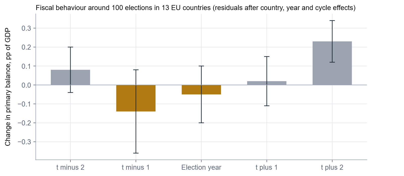
The pattern has a clear shape. Two years before an election, primary balances are on average slightly tighter than normal, by 0.08 points. In the year before the election they loosen by 0.14 points and in the election year by a further 0.05 points. The year after the election is neutral. The correction comes in the second year after the election, when primary balances tighten by 0.23 points relative to normal, the only effect in the event study that is clearly distinguishable from zero. Governments spend before the vote and their successors, or they themselves, consolidate once the new mandate is secure.
3. Italy's Exceptional Cycle
The average effect hides large differences between countries. To measure them, the paper computes an electoral cycle intensity index for each country: the average residual change in the primary balance in election and pre-election years minus the average residual change in all other years. A negative value means that a country's budgets loosen around elections relative to its own behaviour in other years and relative to what other European countries were doing at the same time.
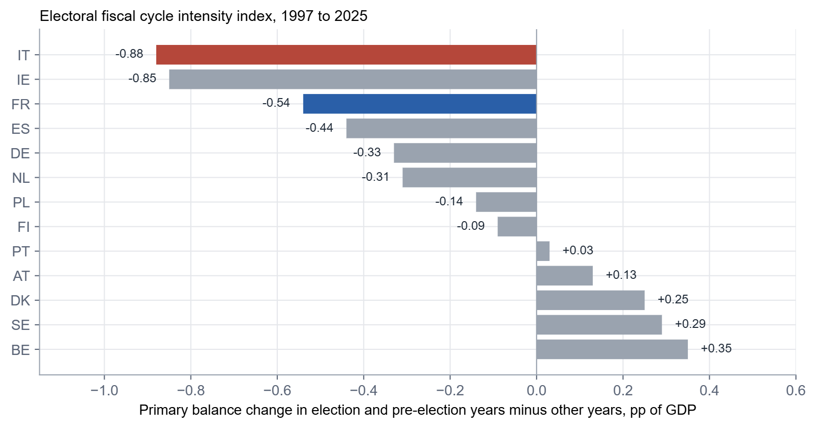
Italy comes first (Figure 4 and Table 4). In election and pre-election years its primary balance moves 0.88 points of GDP worse than in other years. The difference is significant at the 10 per cent level despite the small number of observations, twelve electoral years against seventeen other years. Ireland comes second with a similar point estimate but far more noise, reflecting the violence of its banking crisis. France is third at 0.54 points and is the only country where the difference is significant at the 5 per cent level. Spain, Germany and the Netherlands show smaller cycles of 0.3 to 0.4 points. At the other end, Belgium, Sweden, Denmark and Austria show no electoral loosening at all; if anything they tighten slightly in electoral years.
Table 4. Electoral fiscal cycle intensity index by country
| Country | Index, pp of GDP | t statistic | Electoral years |
|---|---|---|---|
| Italy | minus 0.88 | minus 1.78 | 12 |
| Ireland | minus 0.85 | minus 0.48 | 13 |
| France | minus 0.54 | minus 2.43 | 13 |
| Spain | minus 0.44 | minus 0.83 | 15 |
| Germany | minus 0.33 | minus 1.22 | 16 |
| Netherlands | minus 0.31 | minus 1.19 | 19 |
| Poland | minus 0.14 | minus 0.35 | 13 |
| Finland | minus 0.09 | minus 0.20 | 14 |
| Portugal | plus 0.03 | plus 0.05 | 19 |
| Austria | plus 0.13 | plus 0.26 | 16 |
| Denmark | plus 0.25 | plus 0.54 | 16 |
| Sweden | plus 0.29 | plus 0.70 | 14 |
| Belgium | plus 0.35 | plus 0.76 | 14 |
Note: Residuals from a regression of the annual change in the primary balance on country and year fixed effects, the growth deviation and the lagged primary balance, 1997 to 2025. Welch t statistic for the difference in means. Electoral years count election and pre-election years.
The ranking is suggestive. The Nordic countries, with strong independent fiscal councils, multi-year expenditure ceilings and a tradition of consensual coalition government, show no cycle. Belgium and Austria, with their tradition of long coalition negotiations and federal or social-partner bargaining, show none either. The countries at the top of the ranking, Italy and France, share a political system that rewards the incumbent for visible, concentrated benefits, and a budget process in which the annual finance law is the main instrument of political competition.
The Italian index is also a reminder of why the country-only regression in Section 2.1 failed. Italian budgets do not loosen before elections in absolute terms in every case; they loosen relative to what the rest of Europe is doing in the same year. In 2012, for example, the Italian primary balance improved by 1.0 point before the 2013 election, but Europe as a whole was tightening much harder under market pressure, so Italy's residual is negative. The electoral cycle is visible only when the common European fiscal stance is taken out.
3.1 The pattern applied to 2027
If the panel model is taken at face value, what does it predict for Italy in 2027? Using the full-sample coefficients, an election year with growth of 0.8 per cent, below Italy's long-run average, and a lagged primary surplus of about 0.9 per cent of GDP gives a predicted change in the primary balance of minus 0.48 points of GDP. The government's own plan implies a primary surplus of about 1.0 per cent of GDP in 2026 and 0.5 per cent in 2027, a loosening of 0.5 points.
The match is almost exact, and it is the central finding of this part of the paper. The 2027 budget is not an aberration. It is what Italian and European governments have typically done in election years, at the scale they have typically done it. The escape clause did not create the loosening; it provided a legal channel for it.
What is different from the past is the timing. In the typical Italian cycle the loosening is spread over the pre-election year and the election year. This time the year before the election, 2026, has been a year of tightening: the primary surplus rises from 0.7 per cent of GDP in 2025 to about 1.0 per cent, because the government needed a deficit below 3 per cent to leave the excessive deficit procedure. The electoral loosening has been compressed into a single year and delivered through a European mechanism rather than through a breach of the rules. The European framework has changed the form of the Italian electoral cycle, not its size.
4. What a Euro of Italian Deficit Buys
Whether an electoral loosening is costly depends on what it buys. If extra spending raises output strongly, part of it pays for itself through higher tax revenue, and the debt ratio rises less than the deficit suggests. If the multiplier is low, the deficit goes almost entirely into debt. For Italy the question is pressing, because the 2027 package is concentrated on two kinds of spending, energy transfers and defence, whose effects on output are not obvious.
4.1 Identifying fiscal shocks
The standard approach to measuring fiscal multipliers with time series, introduced by Blanchard and Perotti (2002), uses quarterly data and the fact that governments cannot adjust spending within a quarter in response to unexpected changes in output. Budget decisions take time to make and implement. Any correlation between spending and output within the quarter must therefore run from spending to output. Tax revenue, by contrast, responds automatically to output through the tax system, so its within-quarter correlation with output has to be purged of that automatic response, using an external estimate of the output elasticity of revenue.
The paper estimates a three-variable vector autoregression for Italy with real government spending, real tax revenue and real GDP, in log differences, with four lags, from the first quarter of 1999 to the second quarter of 2026. The pandemic quarters from 2020 to the first quarter of 2021 are controlled for with dummy variables. The output elasticity of revenue is set at 1.0, close to the estimates of the OECD and the European Commission for Italy, and the results are tested for elasticities from 0.7 to 1.3. Two measures of spending are used. The first is real government consumption from the national accounts: public wages and purchases of goods and services, about 20 per cent of GDP. The second is total government expenditure deflated by the GDP deflator: consumption plus social transfers, subsidies, investment and interest, about 50 per cent of GDP. The difference between the two tells us how much transfers and subsidies move output relative to direct purchases.
Multipliers are computed as cumulative multipliers: the cumulative change in GDP over a given horizon divided by the cumulative change in spending or revenue over the same horizon, converted from percentage changes into euros using sample averages of the spending and revenue ratios. This measure, recommended by Ramey (2016), answers the policy question directly: how many euros of GDP does a euro of spending produce over two years? Confidence bands come from 500 bootstrap replications.
4.2 Three multipliers, three orders of magnitude
The results separate clearly into three groups (Figure 5 and Table 5).

A euro of government consumption raises GDP by 0.13 euros in the quarter it is spent, by 0.67 euros after one year and by 0.69 euros after two years. The bootstrap median is somewhat higher, 0.96, and the 68 per cent band is wide, from about zero to 2.0. This is in line with the European literature, which finds government consumption multipliers between 0.5 and 1.0 in normal times for large euro area economies. It is a reasonable central estimate for Italy, and the uncertainty is a reminder that the effect of public purchases depends on the state of the economy and on monetary policy.
A euro of tax increase lowers GDP by 0.09 euros in the first quarter, by about 0.2 euros after one year and by 0.13 euros after two years in the point estimate, with a bootstrap median of 0.27 and a band of 0.07 to 0.50. Tax multipliers in Italy are therefore small. This reflects the structure of the Italian tax system, where a large share of revenue comes from social contributions and consumption taxes that change little with discretionary policy, and the fact that many tax changes are temporary or offset elsewhere.
A euro of total government spending raises GDP by only 0.03 to 0.08 euros at any horizon, with a band from slightly below zero to 0.19. The contrast with government consumption is striking. Since total spending includes government consumption, the near-zero multiplier on the total implies that the other components, social transfers, subsidies and interest payments, have an output effect close to zero in the Italian data. Part of this is mechanical, because interest payments, which go largely to domestic banks, insurers and foreign investors, have little effect on demand. But part reflects the behaviour of transfers: in Italy, a large share of social spending is pensions, which are paid regardless of the cycle, and much of the rest is bonuses and tax credits whose effect on spending is diluted by saving, imports and leakage.
Table 5. Italian fiscal multipliers, euros of GDP per euro
| Instrument | Impact | 4 quarters | 8 quarters | 68% band, 8 quarters |
|---|---|---|---|---|
| Government consumption | 0.13 | 0.67 | 0.69 | minus 0.02 to 2.02 |
| Tax revenue (output loss per euro raised) | 0.09 | 0.19 | 0.13 | 0.07 to 0.50 |
| Total government expenditure | 0.03 | 0.06 | 0.04 | minus 0.08 to 0.19 |
Note: Cumulative multipliers from a three-variable structural VAR in log differences with four lags, 1999 Q1 to 2026 Q2, pandemic dummies, output elasticity of revenue 1.0. Bands from 500 bootstrap replications.
4.3 How robust are these numbers?
Fiscal multipliers are notoriously fragile, and the paper checks the results in three ways (Figure 6).

First, the sample. Before the pandemic, from 1999 to 2019, the government consumption multiplier is somewhat larger, 0.94, and the tax and total expenditure multipliers are also larger, 0.35 and 0.12. Including the pandemic and energy years lowers all three. In the shorter sample from 2008 to 2026, dominated by two crises, the government consumption multiplier jumps to 3.6, a number that reflects the coincidence of austerity and recession in 2011 to 2013 rather than a stable relationship, and should not be used for policy. The tax and total expenditure multipliers, by contrast, barely change across samples.
Second, the lag length. With two lags the multipliers are larger, 1.27 for government consumption and 0.41 for total spending; with six lags they are close to the baseline, 0.79 and 0.24. The ranking never changes: government consumption always has the largest effect, total expenditure the smallest, and the gap between them is always large.
Third, the elasticity of revenue. The government consumption multiplier does not depend on it. The tax multiplier does: with an elasticity of 0.7 it is close to zero, with 1.3 it rises to 0.39. Whatever the exact value, Italian tax multipliers are well below one.
The robust conclusion is not a precise number but a ranking. In Italy, public purchases of goods and services and public employment have a meaningful effect on output, of the order of 0.7 to 1.0 euros per euro over two years. Taxes have a modest effect, of the order of 0.1 to 0.4. Transfers and subsidies, taken together with interest, have almost none.
5. The Growth Arithmetic of the 2027 Budget
These multipliers can be applied to the 2027 package. The exercise requires assumptions about each block, which Table 6 sets out.
Energy relief consists mainly of bonuses on household energy bills, tax credits for energy-intensive firms and support for public buildings. These are transfers and subsidies. The paper assigns them a multiplier of 0.15, at the upper end of the total-expenditure band and roughly twice the point estimate, to allow for the fact that energy support to low-income households has a higher propensity to be spent than the average transfer.
Defence spending is a mix of personnel, operations and equipment. The personnel and operations components behave like government consumption, but equipment is heavily imported: Italian procurement relies on European and American platforms and components, and the import share of defence equipment in large European countries is commonly estimated at 40 to 50 per cent. The paper applies the government consumption multiplier of 0.69 with a 45 per cent import leakage, giving 0.38.
Measures for families and the income tax cut are treated as tax cuts with the estimated tax multiplier of 0.13. Other spending, a mix of public wages, health and investment, is given the average of the consumption and tax multipliers, 0.41. On the financing side, the tax on banks and insurers is given half the tax multiplier, 0.06, because it falls on profits, a large part of which accrues to shareholders abroad or would have been retained; the spending cuts are given 80 per cent of the consumption multiplier, 0.55, because they fall on ministry budgets for goods and services; other covers are given the tax multiplier.
Table 6. Estimated effect of the 2027 budget on GDP
| Block | EUR billion | Multiplier | GDP effect, EUR billion |
|---|---|---|---|
| Energy relief (escape clause) | 7.2 | 0.15 | plus 1.08 |
| Defence (escape clause) | 7.2 | 0.38 | plus 2.73 |
| Families and income tax | 5.0 | 0.13 | plus 0.65 |
| Other spending | 5.0 | 0.41 | plus 2.05 |
| Banks and insurers | minus 5.0 | 0.06 | minus 0.32 |
| Ministry spending cuts | minus 3.5 | 0.55 | minus 1.93 |
| Other covers | minus 1.5 | 0.13 | minus 0.20 |
| Total | 14.4 net | plus 4.06, about 0.16% of GDP | |
| Of which escape clause | 14.4 | 0.26 average | plus 3.81, about 0.15% of GDP |
Note: Multipliers from Table 5 adjusted as described in the text. Nominal GDP in 2027 taken as 2,470 billion euros. Effects are cumulative over 2027 and 2028.
The results are shown in Figure 7. The escape-clause spending of 14.4 billion euros raises GDP by about 3.8 billion euros, 0.15 per cent of GDP. Most of the effect comes from defence, despite the import leakage, because government purchases are the one instrument with a meaningful multiplier. Energy relief, half the money, delivers less than a third of the effect. The ordinary part of the budget is roughly neutral for growth: the 10 billion euros of tax cuts and spending add about 2.7 billion euros of GDP, but the 10 billion euros of covers subtract about 2.5 billion euros, mostly through the spending cuts.

Taken together, the budget adds about 0.16 per cent to GDP over 2027 and 2028. The government forecasts real growth of 0.8 per cent in 2027. On these estimates, the budget accounts for about a fifth of that growth. The rest depends on exports, investment financed by the last year of the recovery plan, and private consumption, which in turn depends on the path of energy prices and real wages discussed elsewhere in this series.
5.1 Cents on the euro
The most useful single number is the output return on the borrowed money. Every euro of escape-clause deficit buys about 26 cents of GDP. Every euro of GDP created costs about 3.8 euros of additional deficit. And because Italian general government revenue is about 48 per cent of GDP, the extra output brings back about 12 cents per euro of tax revenue: only about 13 per cent of the escape-clause deficit finances itself.
This is not an argument against defence or energy spending as such. Both may be justified on strategic grounds, and energy support may prevent social hardship and business failures whose costs do not show up in a multiplier. It is an argument against presenting the escape clause as a growth policy. The clause buys security and relief, perhaps, but almost no growth, and its cost goes almost entirely into debt.
5.2 What a better composition would have bought
The same arithmetic shows what the money could have done. If the 14.4 billion euros had been spent on domestic public purchases and investment with the government consumption multiplier of 0.69 and no import leakage, the GDP effect would have been about 9.9 billion euros, 0.4 per cent of GDP, more than two and a half times the actual effect. If it had been spent entirely on transfers with the estimated total-expenditure multiplier, the effect would have been less than 1 billion euros. The composition of the escape-clause spending, roughly half transfers and half partly imported equipment, places it closer to the bottom of this range than the top.
The European rules shape this composition. The escape clause covers only defence and, in its 2026 extension, energy security; it does not cover public investment in general, education or research, which have higher multipliers. The clause therefore steers deficit spending towards categories where Italian output responds least. It is a fiscal rule designed for strategic purposes, and it should be judged on those purposes, not on its macroeconomic effect.
6. The Debt Legacy
In the years of low interest rates, a temporary deficit faded from the debt ratio over time, because nominal growth exceeded the interest rate. The second paper in this series showed that this is no longer the case for Italy. The marginal cost of new Italian debt, about 3.5 per cent including the spread over Bunds, now exceeds nominal growth of 2.5 to 3 per cent. In these conditions a deficit added today does not shrink as a share of GDP; it grows slowly.
6.1 Ten years of the escape clause
The paper traces the effect of the escape-clause borrowing on the debt ratio from 2027 to 2036, assuming 0.6 points of GDP of extra deficit in each of 2027 and 2028, a marginal cost of borrowing of 3.5 per cent and nominal growth of 2.8 per cent (Figure 8). The small growth effect estimated in Section 5 is ignored, because it reduces the debt ratio by less than 0.1 point.

The extra debt reaches 1.2 points of GDP at the end of 2028. It then does not decline. Because the interest rate exceeds nominal growth, the extra debt rises slowly, to 1.27 points of GDP in 2036. By then it costs about 1.4 billion euros a year in interest, every year, for as long as it is outstanding. The escape clause is temporary; its debt is not.
Table 7. Costs and returns of the escape clause
| Item | Value |
|---|---|
| Extra deficit, 2027 and 2028 | 0.6% of GDP each year, about 14 billion euros a year |
| GDP effect | about 0.15% of GDP, 3.8 billion euros |
| Output per euro of extra deficit | about 0.26 euros |
| Share of the deficit recovered through revenue | about 13% |
| Additional debt ratio, 2028 | 1.20 pp of GDP |
| Additional debt ratio, 2036 | 1.27 pp of GDP |
| Additional interest bill, 2036 | about 1.4 billion euros a year |
| Spread effect, at 2 to 4 basis points per point of debt | 2.4 to 4.8 basis points |
Note: Author's calculations. Spread sensitivity from the range of estimates in the empirical literature on euro area sovereign spreads.
6.2 The market channel
Higher debt also affects the spread. Empirical studies of euro area sovereign spreads, including those surveyed by the European Commission and the ECB, find that each percentage point of debt to GDP raises the long-term spread by 2 to 4 basis points, more in periods of stress. On that basis, the 1.2 points of escape-clause debt add 2.4 to 4.8 basis points to the BTP-Bund spread. That is small compared with the 50 basis points of widening in 2026, but it is permanent, and it applies to the entire stock as it is refinanced.
The bigger risk is not the arithmetic effect but the signal. The second paper in this series showed that the fragility frontier, the spread at which the Italian debt ratio stops rising, is about 60 basis points with a primary surplus of 0.5 per cent of GDP, and about 100 basis points with a surplus of 1 per cent. With the spread at 112 to 117 basis points in early November, Italy is already on the wrong side of the line in 2027. Markets have so far treated the 2026 widening as a repricing, not a stress episode. They will watch whether the escape clause is followed, from 2029, by the consolidation the government promises, or whether a new government finds new reasons to postpone it.
7. The European Dimension
The escape clause raises questions for Brussels as well as for Rome. The reformed European fiscal framework, in force since 2024, replaced the old structural balance targets with a single operational indicator: the growth of net primary expenditure, agreed in a medium-term plan. The national escape clause allows a member state to deviate from that path for defence, and now energy security, up to a ceiling. The design assumes that these deviations are temporary and strategically motivated.
The Italian case tests both assumptions. On timing, the evidence in Sections 2 and 3 shows that Italy's use of the clause coincides with the electoral calendar and replicates, almost exactly, the loosening that Italian governments have historically delivered in election years. On motivation, roughly half of the Italian allowance goes to energy relief, a category that is closer to social policy than to strategic investment. None of this is a violation of the rules. It shows how a framework built around strategic exemptions can be used to accommodate domestic political cycles.
There is also a question of consistency. The government's argument that the deficit net of the clause, 2.8 per cent in 2027, is what matters for the excessive deficit procedure is legally sound under the new rules if the Council confirms the activation. But markets and rating agencies look at the headline deficit and the debt ratio. A country can leave the excessive deficit procedure while its headline deficit is above 3 per cent and its debt ratio is rising, as the government's own projections show: 138.1 per cent of GDP in 2026, 138.6 per cent in 2027, falling only from 2028. The procedure will say one thing, the numbers another.
8. Arguments on Both Sides
The case for the 2027 budget deserves a fair statement. Its defenders make four arguments.
First, the energy shock is real and severe. Italian inflation was 5.6 per cent in October 2026, the highest among large euro area economies, driven almost entirely by energy, as the first paper in this series showed. Households and energy-intensive firms face genuine hardship, and support for them is a legitimate use of public money, especially when the cause is an external shock that no Italian policy could have prevented.
Second, defence spending is a European obligation. Italy has committed with its NATO allies to raise defence spending substantially over the coming decade. It cannot do so within its ordinary budget without cuts elsewhere that would be socially and politically unsustainable. The escape clause exists precisely to allow this transition.
Third, Italy's fiscal record since 2023 is strong. The deficit has been cut from 7.1 per cent of GDP in 2023 to an expected 2.9 per cent in 2026, a consolidation of more than four points in three years, larger than that of almost any other large European country. The primary balance is back in surplus. A government that has done this much can reasonably use the flexibility that the rules provide.
Fourth, the scale is modest. Half a point of GDP of loosening is small compared with the pandemic and energy packages of 2020 to 2023, and the ordinary part of the budget is roughly neutral.
These arguments have force, and the paper does not dispute them. Its findings bear on a narrower point. If the purpose of the extra spending is relief and security, it should be presented and judged as such, and the cost should be recognised. The multipliers estimated here suggest that the cost is close to the full amount borrowed, that the growth return is small, and that the debt will remain after the election and after the clause has expired. The critics' case is not that the budget is reckless; it is that it repeats a familiar pattern at a moment when the arithmetic of debt has turned against Italy.
9. Policy Implications
Several practical implications follow.
- Judge the escape clause by its purpose, not by its growth effect. The output return of about 26 cents per euro means that the clause cannot be defended as stimulus. It can be defended as insurance against energy hardship and as an investment in security. Communicating it that way would be more honest and would set realistic expectations for 2027 growth.
- Shift the composition towards domestic purchases and targeted support. Within the energy envelope, support targeted at low-income households and at investment in efficiency has higher output effects than general bill subsidies. Within defence, a larger domestic share of procurement, where industrial capacity exists, would raise the multiplier. Both changes are compatible with the clause.
- Commit to the post-election consolidation now. The government's plan has the primary surplus rising to 1.8 per cent of GDP from 2029. Markets will discount this path heavily unless it is anchored in law. A multi-year expenditure ceiling, binding on the next government and monitored by the Ufficio parlamentare di bilancio, would make the promise credible.
- Strengthen fiscal institutions against the electoral cycle. The countries with the smallest electoral cycles in the panel, the Nordic countries, Belgium and Austria, share strong independent fiscal councils and multi-year budget frameworks. Italy has the institutions on paper. Giving the parliamentary budget office a formal role in assessing electoral-year budgets, and publishing a cycle-adjusted measure of the fiscal stance, would raise the political cost of loosening.
- Make the European clause conditional on composition. At the European level, the escape clause could be restricted to spending with demonstrated strategic or investment value, and energy relief could be required to be targeted and temporary. That would reduce the scope for using a strategic exemption to finance a generic electoral budget.
10. Conclusions
The 2027 Italian budget is a European-sanctioned version of an old Italian habit. The panel evidence shows that Italy has the strongest electoral fiscal cycle of thirteen EU countries over three decades, with primary balances deteriorating by almost one point of GDP around elections relative to other years and to European peers. The 2027 budget loosens the primary balance by half a point, exactly what the historical model predicts for an election year. The novelty lies in the channel: the escape clause for defence and energy security allows the loosening without breaching the rules and, if the 2026 deficit is confirmed, while leaving the excessive deficit procedure.
The macroeconomic return on this borrowing is low. Italian fiscal multipliers, estimated with a structural VAR on 27 years of quarterly data, are about 0.7 for government purchases, 0.1 to 0.3 for taxes and close to zero for spending that includes transfers. Applied to the composition of the escape-clause spending, they imply that each euro of extra deficit buys about 26 cents of GDP, and that the budget as a whole adds about 0.16 per cent to output. Because the interest rate on new Italian debt now exceeds nominal growth, the 1.2 points of GDP borrowed in 2027 and 2028 will still be on the books, slightly larger, in 2036.
None of this makes the budget irresponsible. The amounts are modest, the energy shock is real and the defence commitments are shared across Europe. But the paper's findings point to a structural problem. Italy's fiscal framework, domestic and European, still allows electoral cycles to shape the budget, and the new European rules have given those cycles a respectable form. In a world of low interest rates the cost was small. In the world of 2026, where every point of deficit stays as debt, it is not.
Appendix: Methods and Robustness
A.1 Panel specification
The panel regression is estimated on the annual change in the primary balance, defined as the general government balance (B9) plus interest payable (D41), both in per cent of GDP, for thirteen countries from 1997 to 2025. Election years are years in which a national legislative election was held; where two elections took place in the same year, as in Spain in 2019, the year counts once. Pre-election years are the calendar years before an election, and post-election years the calendar years after. The growth deviation is real GDP growth minus the country's 1996 to 2025 average. Standard errors are clustered by country; with thirteen clusters they should be read as approximate.
A.2 Structural VAR
The VAR includes the log differences of real government spending, real tax revenue and real GDP, with four lags, a constant and dummy variables for each quarter from 2020 Q1 to 2021 Q1. Real revenue is total general government revenue divided by the GDP deflator. Identification follows Blanchard and Perotti (2002): spending does not respond to output or revenue within the quarter; revenue responds to output with an elasticity of 1.0 and to spending with a coefficient estimated from the cyclically adjusted revenue residual; output responds to both, with coefficients estimated by instrumental variables using the structural spending and revenue shocks as instruments. The estimated within-quarter response of revenue to spending is minus 0.20.
Table A1. Sensitivity of eight-quarter cumulative multipliers
| Specification | Government consumption | Taxes | Total expenditure |
|---|---|---|---|
| Baseline, 1999 Q1 to 2026 Q2, 4 lags, elasticity 1.0 | 0.69 | 0.13 | 0.04 |
| Sample 1999 Q1 to 2019 Q4 | 0.94 | 0.35 | 0.12 |
| Sample 2008 Q1 to 2026 Q2 | 3.57 | 0.30 | 0.14 |
| 2 lags | 1.27 | 0.34 | 0.41 |
| 6 lags | 0.79 | 0.49 | 0.24 |
| Revenue elasticity 0.7 | 0.69 | minus 0.09 | 0.04 |
| Revenue elasticity 1.3 | 0.69 | 0.39 | 0.04 |
| Bootstrap median, baseline | 0.96 | 0.27 | 0.06 |
Note: Tax multiplier expressed as output loss per euro of revenue raised; a negative value means output rises after a tax increase. The 2008 to 2026 estimate for government consumption is driven by the 2011 to 2013 episode and is not used.
A.3 Debt simulation
The debt legacy is computed recursively: the additional debt ratio in each year equals the previous year's additional ratio multiplied by the ratio of one plus the marginal cost of borrowing to one plus nominal growth, plus any additional deficit in that year. The marginal cost of borrowing, 3.5 per cent, equals a Bund yield of 3.2 per cent plus a spread of 115 basis points minus the Treasury's average term discount of 0.84 points estimated in the second paper of this series. With a lower marginal cost of 3.0 per cent, the additional debt ratio in 2036 is 1.22 points rather than 1.27; with 4.0 per cent it is 1.32.
References
Blanchard, O. and Perotti, R. (2002). An empirical characterization of the dynamic effects of changes in government spending and taxes on output. Quarterly Journal of Economics, 117(4), 1329 to 1368.
Brender, A. and Drazen, A. (2005). Political budget cycles in new versus established democracies. Journal of Monetary Economics, 52(7), 1271 to 1295.
Council of the European Union (2024). Regulation (EU) 2024/1263 on the effective coordination of economic policies and on multilateral budgetary surveillance. Brussels.
European Commission (2025). Communication on accommodating increased defence expenditure within the Stability and Growth Pact. Brussels, March 2025.
Eurostat (2026). Government deficit and debt (gov_10dd_edpt1); quarterly non-financial accounts for general government (gov_10q_ggnfa); national accounts (nama_10_gdp, namq_10_gdp). Luxembourg.
Italian Government (2026). Documento programmatico di finanza pubblica 2026, 2 October 2026; Documento programmatico di bilancio 2027, 13 October 2026. Rome: Ministero dell'Economia e delle Finanze.
Nordhaus, W. D. (1975). The political business cycle. Review of Economic Studies, 42(2), 169 to 190.
Ramey, V. A. (2016). Macroeconomic shocks and their propagation. In Handbook of Macroeconomics, Vol. 2, 71 to 162. Amsterdam: Elsevier.
Rogoff, K. (1990). Equilibrium political budget cycles. American Economic Review, 80(1), 21 to 36.
Ufficio parlamentare di bilancio (2026). Audizione sul Documento programmatico di finanza pubblica 2026. Rome: UPB.
Driss EFFINA, PhD
Independent Researcher, Global Strategy Files
The opening pages of our four country reports: United States, United Kingdom, Japan and China. A free PDF, sent to your inbox.
You will also receive occasional analysis from Global Strategy Files. Unsubscribe in one click, at any time.