The Creditor That Cannot Collect: Student Loan Defaults, the Atrophy of Federal Collections and the 2027 Cash-Flow Shock

Abstract
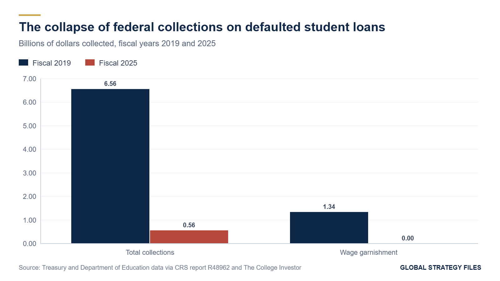
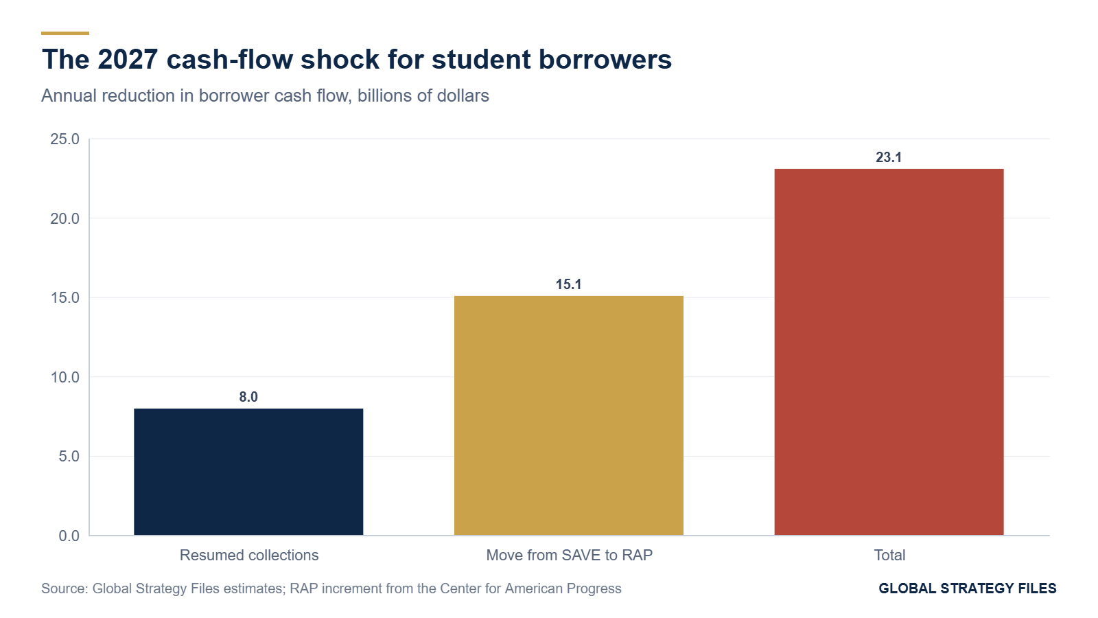
The federal government is the largest consumer lender in the United States. It holds about 1.7 trillion dollars of student loans owed by about 43 million borrowers, more than the outstanding balance of all credit cards. In 2026 this lender faces a crisis of a peculiar kind: not a crisis of solvency, but a crisis of collection. The number of borrowers in default on federally managed loans rose from 5.2 million in September 2025 to 9.3 million in June 2026, and defaulted loans now represent about 14 percent of federal student debt, against 12.5 percent before the pandemic. At the same time, the machinery for recovering defaulted debt has almost stopped. Collections on defaulted loans fell from 6.56 billion dollars in fiscal year 2019 to 560 million in fiscal 2025, and administrative wage garnishment, which brought in 1.34 billion dollars in 2019, collected about 510,000 dollars in 2025. Involuntary collections were paused again in January 2026, and responsibility for defaulted loans was transferred to the Treasury in March. This study reconstructs twenty years of student debt, delinquency and default, measures the collapse of the government's recovery yield, and projects defaults and cash flows to the end of 2028 with a stock-flow model under three scenarios. We find that the implied annual recovery yield on defaulted balances fell from about 3.5 percent before the pandemic to about 0.3 percent in 2025, an eleven-fold decline. Our projections put the number of borrowers in default at between 8.2 and 11.0 million at the end of 2028, depending on the vigor of collections and on the payment shock created by the new Repayment Assistance Plan. We show that the restart of collections in 2027 would withdraw about 8 billion dollars a year from household budgets, and the transition from the SAVE plan to the new repayment plan about 15 billion dollars more, for a combined cash-flow shock of about 23 billion dollars concentrated on about 16 million borrowers. The macroeconomic effect is small, about 0.03 percent of consumption for collections alone, but the distributional effect is large: a garnished worker with 3,100 dollars of monthly disposable pay loses about 5,580 dollars a year.
Key findings
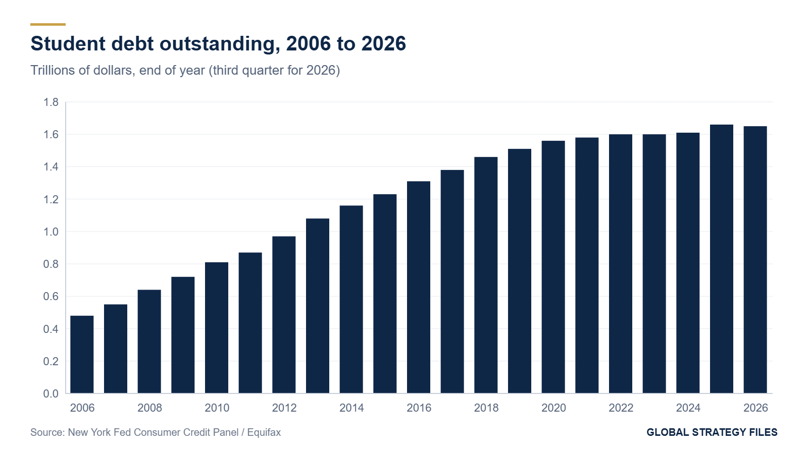
- Student debt rose from about 0.48 trillion dollars in 2006 to about 1.65 trillion in 2026, and became the second largest category of household debt after mortgages.
- The flow of student balances into serious delinquency, near zero during the payment pause of 2020 to 2024, jumped to 14.3 percent in the third quarter of 2025, the highest on record, before easing to 7.7 percent in the third quarter of 2026.
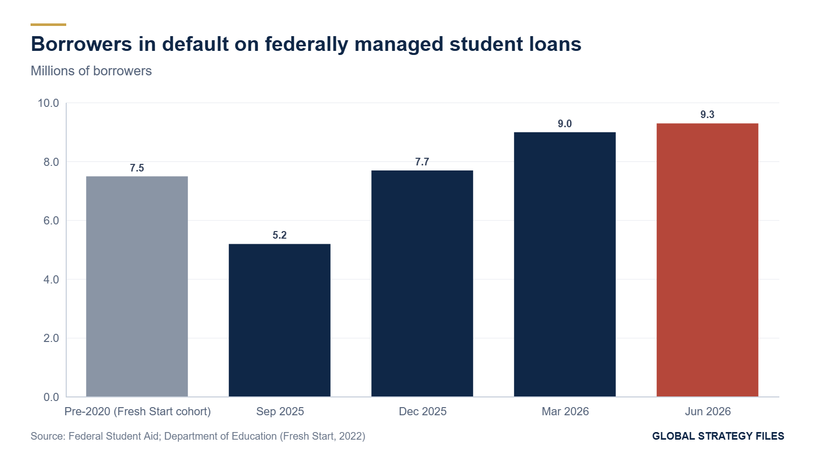
- Borrowers in default rose by 4.1 million in nine months, from 5.2 million to 9.3 million. In December 2025 the default rate was identical to 2019; the entire increase above the pre-pandemic norm occurred in the first half of 2026.
- The recovery yield of federal collections fell from about 3.5 percent of defaulted balances a year in 2019 to about 0.3 percent in 2025.
- By the end of 2028, defaults would stand at about 9.3 million under a managed scenario, 8.2 million under vigorous enforcement and 11.0 million under a stress scenario.
- In 2027, the combined effect of resumed collections and higher payments under the Repayment Assistance Plan would reduce the cash flow of student borrowers by about 23 billion dollars, twice as much from the plan transition as from collections.
1. Introduction: a lender that stopped collecting
Every lender faces defaults. What distinguishes a functioning lender from a failing one is not the absence of default but the capacity to recover. A bank that lends to households expects to lose a predictable share of its loans and to recover part of the loss through collections, settlements and the sale of claims. The federal student loan program was designed on the same principle, with unusually powerful tools: the government can garnish up to 15 percent of a defaulted borrower's disposable pay without a court order, seize federal tax refunds, and offset part of Social Security benefits. These tools made federal student loans among the hardest debts to escape in American law.
Between March 2020 and 2026, these tools were almost entirely unused. The pandemic pause on payments and collections lasted until September 2023. A one-year on-ramp protected late borrowers from the worst consequences until September 2024. Collections through the Treasury Offset Program restarted in May 2025, and the Education Department announced that wage garnishment would resume, but in January 2026 it paused involuntary collections again to prepare the transition to the repayment plans created by the 2025 budget law. In March 2026, an interagency agreement transferred responsibility for defaulted loans to the Treasury, which has signaled that it will rely on private collection agencies, possibly hired from November 2026, with garnishment and refund seizures more likely to resume in 2027.
Meanwhile, defaults have surged. This study asks three questions. How large and how unusual is the 2025 to 2026 wave of defaults in a twenty-year perspective? How far has the government's capacity to recover defaulted debt deteriorated? And what will happen to defaults, to collections and to household cash flows when the machinery restarts? Section 2 reconstructs the long history of student debt and delinquency. Section 3 documents the default wave. Section 4 measures the collapse of collections. Section 5 presents a stock-flow model of default and projects it to 2028. Section 6 estimates the cash-flow shock of 2027. Section 7 draws the implications.
2. Twenty years of student debt
2.1 From 0.5 to 1.65 trillion dollars
In 2006, Americans owed about 480 billion dollars in student loans, roughly half of what they owed on auto loans. By 2012 student debt had passed one trillion dollars, overtaking credit cards and auto loans to become the second largest category of household debt. Figure 1 shows the trajectory. Growth was fastest in the years after the financial crisis, when enrollment rose, tuition increased faster than incomes and the federal government became, after 2010, the direct lender for almost all new student loans. Growth slowed in the late 2010s and stopped almost entirely during the pause, when interest was set to zero on federally held loans. In 2025 and 2026 the balance stabilized near 1.65 trillion dollars, as payments resumed and new borrowing slowed.
The structure of the debt has changed as much as its size. In 2006, most student loans were guaranteed loans made by private lenders under the Federal Family Education Loan program. Since 2010, new federal loans have been made directly by the Education Department. The government is therefore not only the guarantor but the creditor, and every dollar not repaid is a dollar lost to the Treasury.
2.2 Delinquency before, during and after the pause
The New York Fed measures the share of student loan balances that transition into serious delinquency (90 days or more past due) each year. Figure 2 shows an approximate annual series. Before the pandemic, the rate rose from about 6.5 percent in 2006 to a peak of about 11.5 percent in 2013, as the cohorts that borrowed heavily during the recession entered repayment, and then eased to about 9 percent in 2017 to 2019. During the pause, it fell to less than 1 percent, because no payments were due and no delinquencies were reported to credit bureaus.

The return of credit reporting in 2025 produced the largest jump in the history of the series. The quarterly transition rate was 8.0 percent in the first quarter of 2025, 12.9 percent in the second and 14.3 percent in the third, a record. It then declined: 10.9 percent in the first quarter of 2026, 7.8 percent in the second and 7.7 percent in the third. The pattern is that of a stock being worked off: borrowers who had stopped paying during the pause and the on-ramp were reported delinquent in a short window, after which the flow returned toward, and then below, its pre-pandemic level.
2.3 Who defaults
Twenty years of research on student loans have produced a robust and counterintuitive finding: default is concentrated not among borrowers with the largest debts but among those with small balances who did not complete their programs. Borrowers with graduate degrees and six-figure balances default rarely, because their earnings are high. Borrowers who left a community college or a for-profit institution without a credential, owing less than 10,000 dollars, default at much higher rates, because the loan bought no increase in earnings. Studies by Looney and Yannelis, using administrative data, showed that the surge in defaults after the financial crisis was driven by nontraditional borrowers at for-profit and two-year institutions, whose numbers had risen sharply during the recession.
This structure matters for the 2026 wave and for the design of collections. The borrowers most likely to be in default today are disproportionately low earners, many without a degree, many in their thirties and forties, and many who have been out of school for a decade or more. For them, wage garnishment and refund seizures take a share of income that is large relative to their budgets, and the balance owed is often small relative to the administrative cost of collecting it. A collection strategy designed for the average borrower will be badly calibrated for the typical defaulter.
2.4 The credit score channel
The end of the reporting pause in 2025 had an immediate effect on credit scores. When delinquencies on student loans were again reported to credit bureaus in the first months of 2025, the New York Fed found that more than two million borrowers with newly reported delinquencies saw their scores fall by more than 100 points, and about one million by more than 150 points. A fall of this size can move a borrower from prime to subprime territory, raising the cost of auto loans, credit cards and insurance, and complicating rental applications. The default wave of 2026 has extended this damage, because default is reported separately and remains on the credit record for seven years unless the loan is rehabilitated. The credit score channel is the main way in which the student loan crisis spills over into the rest of household finance, and it operates even when the government collects nothing.
3. The default wave of 2025 and 2026
3.1 Nine months, four million borrowers
A federal student loan enters default after 270 days without payment. Because of this lag, the delinquency wave of 2025 became a default wave in late 2025 and 2026. According to Federal Student Aid, the number of borrowers in default on federally managed loans was 5.2 million in September 2025, 7.7 million in December 2025, 9.0 million in March 2026 and 9.3 million in June 2026. Another 1.5 million were in late-stage delinquency, the last step before default. The Center for American Progress put the number at 9.5 million in October 2026, more than one federal borrower in five.
Figure 3 places these numbers in perspective. The pre-pandemic default stock was large: in 2022, the Fresh Start program offered relief to about 7.5 million borrowers in default on federally held and guaranteed loans, most of whom had defaulted before 2020. Fresh Start returned many of them to good standing, which is why the stock had fallen to 5.2 million by September 2025. The wave of 2025 and 2026 has therefore erased the effect of Fresh Start and pushed the stock above its pre-pandemic level. Defaulted loans now account for about 14 percent of federal student debt, against 12.5 percent before the pandemic.
3.2 The timing of the increase
An analysis of the Federal Student Aid data shows that in December 2025 the default rate matched exactly its 2019 level, and that all of the increase above the pre-pandemic norm occurred in the first half of 2026. The timing is significant. It means that the default wave was not simply the mechanical consequence of the end of the pause, which would have produced a return to the old rate; it reflects new defaults among borrowers who had been in repayment or in forbearance during 2025. Three factors contributed. The SAVE plan, which had offered very low payments to about 7.7 million borrowers at its peak, was blocked by the courts and then ended, leaving about 7 million borrowers in a forbearance that did not prevent anxiety or confusion and pushing others into older plans with higher payments. The labor market slowed in 2025, with the weakest job creation outside a recession since 2003. And the administrative capacity of the Education Department was reduced by staff cuts at the moment when demand for servicing was highest.
3.3 The quarterly slowdown
The quarterly increments tell a story of deceleration: plus 2.5 million in the fourth quarter of 2025, plus 1.3 million in the first quarter of 2026, plus about 0.3 to 0.4 million in the second. The flow into serious delinquency fell over the same period. The wave is passing its crest. But the stock it leaves behind is the largest in the history of the program, and it will not shrink without either a recovery of collections or a large program of rehabilitation and consolidation.
4. The collapse of collections
4.1 Six billion dollars to half a billion
The federal government has historically recovered a substantial share of defaulted student loans. In fiscal year 2019, it collected 6.56 billion dollars from defaulted borrowers through voluntary payments, rehabilitation, litigation, wage garnishment and the offset of tax refunds and other federal payments. Administrative wage garnishment alone brought in 1.34 billion dollars. In fiscal year 2025, total collections were about 560 million dollars, a decline of 91 percent, and garnishment collected about 510,000 dollars. Figure 4 shows the comparison.
4.2 The recovery yield
To measure the change in the effectiveness of collection independently of the size of the defaulted portfolio, we compute a recovery yield: annual collections divided by the stock of defaulted balances. Before the pandemic, defaulted loans represented about 12.5 percent of a federal portfolio of about 1.5 trillion dollars, or roughly 190 billion dollars; collections of 6.56 billion dollars imply a yield of about 3.5 percent a year. In 2025, defaulted balances were about 180 billion dollars at the start of 2026 according to Federal Student Aid; collections of 560 million dollars imply a yield of about 0.3 percent. The recovery yield has fallen by a factor of about eleven.
Table 1. The federal student loan collection machine, 2019 and 2025
| Indicator | Fiscal 2019 | Fiscal 2025 | Change |
|---|---|---|---|
| Total collections on defaulted loans (billion dollars) | 6.56 | 0.56 | -91 percent |
| Of which administrative wage garnishment (billion dollars) | 1.34 | 0.0005 | -99.96 percent |
| Defaulted balances (billion dollars, approximate) | 190 | 180 | -5 percent |
| Recovery yield (collections over defaulted balances) | 3.5 percent | 0.3 percent | divided by 11 |
| Borrowers in default (millions) | about 7 to 8 | 5.2 (Sept. 2025) rising to 9.3 (June 2026) |
Source: Department of Education and Treasury data reported by the Congressional Research Service and The College Investor; Federal Student Aid; Global Strategy Files calculations.
4.3 Why collection capacity matters
A low recovery yield is not only a fiscal problem. It also changes incentives. When borrowers observe that default has no immediate consequence beyond a damaged credit score, the cost of default falls, and the share of borrowers who stop paying may rise further. Conversely, a sudden restart of aggressive collection after five years of near inactivity can create a shock for households that had adjusted their budgets to the absence of payments. The transfer of collection to the Treasury creates a further risk: the Treasury has experience with cross-servicing of other federal debts, but its earlier experience with student loans, in the 2010s, was criticized for delays and weak borrower contact, and the private collection agencies it plans to use were the subject of enforcement actions by the Consumer Financial Protection Bureau for misleading borrowers about their options.
5. A stock-flow model of default, 2026 to 2028
5.1 Structure
The number of borrowers in default evolves according to a simple accounting identity: the stock at the end of a quarter equals the stock at the beginning, plus new defaults, minus exits. Exits occur through rehabilitation (nine on-time payments, which remove the default from the credit report), consolidation into a new loan, payment in full, discharge for disability or death, and, in principle, through forgiveness programs. New defaults come from the pool of borrowers in late-stage delinquency, which is itself fed by borrowers who stop paying.
We model the stock of defaulted borrowers D at a quarterly frequency from the third quarter of 2026 to the end of 2028:
D(t+1) = D(t) + F(t) minus e(t) times D(t),
where F(t) is the inflow of new defaults and e(t) the quarterly exit rate. The inflow starts at 300,000 borrowers a quarter, consistent with the increase of 0.3 to 0.4 million in the second quarter of 2026 and with a late-stage delinquent pool of about 1.5 million, and declines geometrically as the post-pause stock is worked off. The exit rate starts at 1 percent a quarter, reflecting the near absence of collection pressure in 2026, and rises when collections resume. Before the pandemic, exits from default through rehabilitation and consolidation were in the order of 8 to 10 percent of the defaulted stock a year, or about 2 to 2.5 percent a quarter.
5.2 Three scenarios
The managed scenario assumes that the Repayment Assistance Plan absorbs most at-risk borrowers, that collections resume gradually in 2027 with an emphasis on rehabilitation, and that the exit rate returns to its pre-pandemic level of 2.5 percent a quarter. The inflow declines by 8 percent a quarter.
The enforcement scenario assumes that wage garnishment and Treasury offsets resume at scale in the first half of 2027, that private collection agencies push borrowers into rehabilitation and consolidation, and that the exit rate rises to 4 to 4.5 percent a quarter in 2027 before easing. The inflow declines by 10 percent a quarter, because the credible threat of collection deters new defaults.
The stress scenario assumes that the transition from SAVE to the Repayment Assistance Plan raises payments sharply for millions of borrowers, that the labor market weakens, and that collections remain disorganized. The inflow starts at 450,000 a quarter and declines only slowly, and the exit rate remains near 2 percent a quarter.
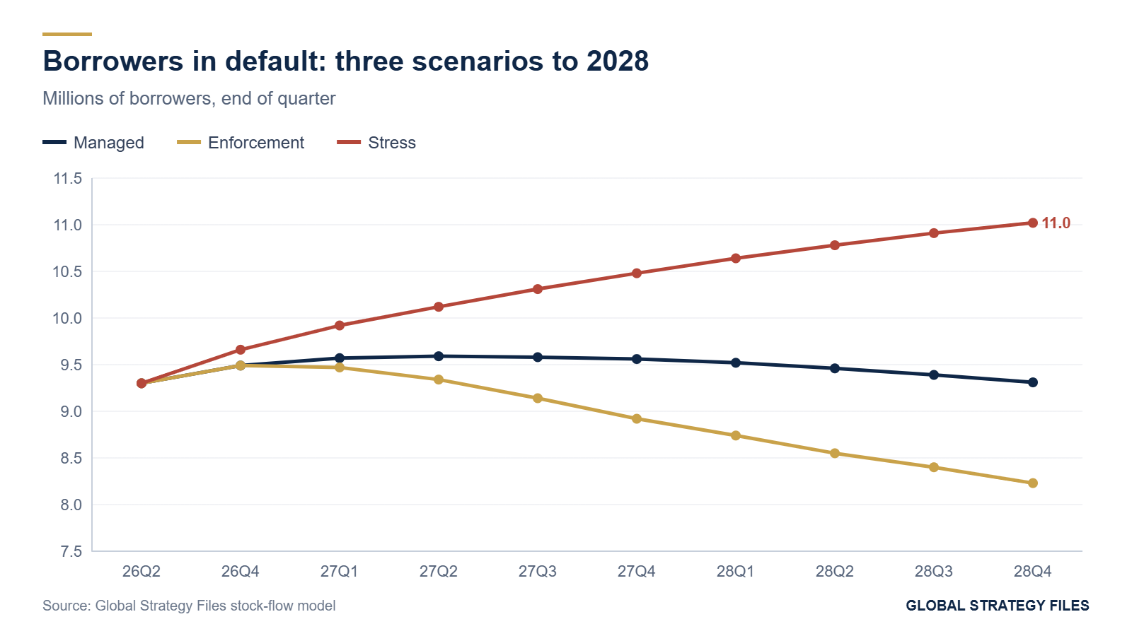
Table 2. Borrowers in default under three scenarios, millions
| End of quarter | Managed | Enforcement | Stress |
|---|---|---|---|
| 2026 Q2 (observed) | 9.3 | 9.3 | 9.3 |
| 2026 Q4 | 9.6 | 9.5 | 9.9 |
| 2027 Q2 | 9.6 | 9.1 | 10.3 |
| 2027 Q4 | 9.5 | 8.7 | 10.6 |
| 2028 Q2 | 9.4 | 8.4 | 10.8 |
| 2028 Q4 | 9.3 | 8.2 | 11.0 |
| Cumulative exits, 2026 Q3 to 2028 Q4 | 2.0 | 2.9 | 1.9 |
Source: Global Strategy Files stock-flow model.
5.3 Interpretation
The scenarios show that the stock of defaults is highly persistent. Even under vigorous enforcement, it remains above 8 million at the end of 2028, about 3 million more than in September 2025. Under the managed scenario, it plateaus near 9.5 million. Under stress, it reaches 11 million, roughly one federal borrower in four. The difference between scenarios is driven more by the exit rate than by the inflow: once borrowers are in default, they stay there unless collection pressure or attractive rehabilitation options pull them out. The policy choices of 2027, and the administrative competence of the Treasury and its contractors, will determine where in this range the program ends.
5.4 What drives the stock: a sensitivity analysis
To identify the parameters that matter most, we varied each assumption of the managed scenario while holding the others constant, and recorded the number of borrowers in default at the end of 2028. Table 3 reports the results. The stock is most sensitive to the exit rate: raising the quarterly exit rate from 2.5 to 3.5 percent lowers the end-2028 stock by about 0.7 million, and lowering it to 1.5 percent raises it by about 0.8 million. A difference of one percentage point in the quarterly exit rate, which is the margin that collection policy and rehabilitation outreach control, is worth roughly 750,000 borrowers. The initial inflow matters too, but less: an inflow of 400,000 a quarter instead of 300,000 raises the stock by about 0.6 million. The speed at which the inflow declines matters least.
Table 3. Sensitivity of the end-2028 default stock to model parameters, managed scenario
| Parameter change | Borrowers in default, end 2028 (millions) | Difference from base |
|---|---|---|
| Base (inflow 300,000, decline 8 percent, exit 2.5 percent) | 9.17 | |
| Exit rate 1.5 percent a quarter | 9.97 | +0.80 |
| Exit rate 2.0 percent | 9.56 | +0.39 |
| Exit rate 3.0 percent | 8.80 | -0.37 |
| Exit rate 3.5 percent | 8.44 | -0.73 |
| Exit rate 4.5 percent | 7.76 | -1.41 |
| Initial inflow 200,000 | 8.58 | -0.59 |
| Initial inflow 400,000 | 9.76 | +0.59 |
| Initial inflow 500,000 | 10.35 | +1.18 |
| Inflow does not decline | 9.85 | +0.68 |
Source: Global Strategy Files stock-flow model; exit rate applied uniformly from 2026 Q3, which explains the small difference with the managed path of Table 2.
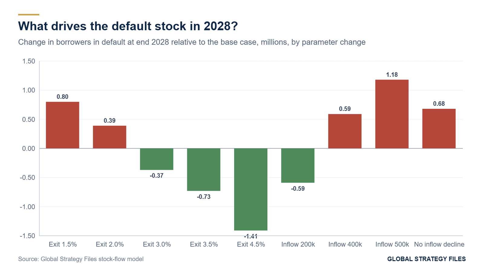
The policy lesson is clear. The number of Americans in default at the end of the decade will depend less on how many more borrowers fall behind than on how effectively the government helps, or forces, those already in default to leave it. Rehabilitation capacity, accurate borrower records and functioning servicers are therefore the decisive variables, more than the generosity of the new repayment plan.
6. The 2027 cash-flow shock
6.1 Collections
If collections return to their pre-pandemic recovery yield of about 3.5 percent of defaulted balances a year, and defaulted balances stand at about 230 billion dollars (14 percent of the federal portfolio), annual collections would be about 8 billion dollars. At a lower yield of 2 percent, they would be about 4.6 billion; at a higher yield of 6 percent, consistent with an aggressive enforcement push, about 14 billion. For an individual worker, a garnishment of 15 percent of disposable pay of 3,100 dollars a month represents about 465 dollars a month, or 5,580 dollars a year. For a family that relies on the Earned Income Tax Credit, the seizure of a refund can represent a quarter or more of annual cash income in a single month. Retirees in default face the offset of part of their Social Security benefits.
6.2 The plan transition
The second source of cash-flow pressure is less visible but larger. The 2025 law replaced the existing income-driven repayment options for new borrowers with the Repayment Assistance Plan, which took effect on 1 July 2026, and ended the SAVE plan. The Center for American Progress estimates that borrowers moving from SAVE to the new plan will pay on average about 2,163 dollars more a year. Applied to about 7 million borrowers who were enrolled in SAVE or in the related forbearance, this represents about 15 billion dollars a year of additional payments, if all of them pay.
6.3 The combined shock
Figure 6 summarizes the two components. Together, resumed collections and the plan transition would reduce the disposable cash flow of student borrowers by about 23 billion dollars a year from 2027. The plan transition accounts for about two thirds of the total. At an assumed marginal propensity to consume of 0.7 for these households, the reduction in consumer spending would be about 16 billion dollars, or 0.08 percent of personal consumption expenditures. Collections alone would subtract about 0.03 percent.
These macroeconomic magnitudes are small. A shock of this size would not, by itself, change the trajectory of the American economy. But the distribution of the shock is highly concentrated. It falls on about 16 million borrowers, disproportionately young adults, people who did not complete their degrees, Black borrowers, and residents of states with lower incomes. For them, the restart of collection is a significant loss of income at a time when real wages are falling and fuel, rent and food costs are high. And because default also damages credit scores, it raises the cost of every other form of credit these households use, from car loans to rental applications.
6.4 The fiscal side
From the government's point of view, the stakes are also modest relative to the budget. Additional collections of 8 billion dollars a year would reduce the 2 trillion dollar deficit by about 0.4 percent. The cost of the program to the government depends far more on the repayment terms of the 1.4 trillion dollars that are not in default than on the recovery of the defaulted portion. The political economy of collection is therefore asymmetric: aggressive collection brings small fiscal gains and large visible costs to specific households, while lax collection brings small fiscal losses and erodes the credibility of the loan program for future borrowers.
7. Implications
Restore capacity before restoring pressure. The collapse of the recovery yield reflects the dismantling of the collection machine over five years, not only the policy pauses. Restarting garnishment through contractors who lack accurate borrower records risks erroneous collections, refunds and litigation, as the Treasury's earlier experience showed. The first priority should be accurate data and functioning rehabilitation channels.
Use the rehabilitation channel as a pressure valve. Rehabilitation requires nine payments based on income, can cost as little as a few dollars a month for low-income borrowers, and removes the default from the credit record. A collection strategy that leads with rehabilitation and uses garnishment only as a last resort would maximize exits from default while minimizing hardship, and our model shows that exits matter more than inflows for the trajectory of the stock.
Sequence the shocks. The plan transition and the restart of collections will hit the same households in the same year. Phasing in the new repayment plan more slowly, or delaying garnishment for borrowers who enroll in an income-driven plan, would spread the shock.
Watch the second-order effects. Defaulted borrowers lose access to federal student aid, which affects older students returning to school, and see their credit scores fall, which affects auto lending, rental markets and employment screening. These effects are not captured in our cash-flow estimates and may be larger than the direct transfers.
Recognize the limits of the asset. The federal student loan portfolio is a financial asset on the government's balance sheet, but it is also a social policy. The tension between the two roles has been papered over by pauses since 2020. The years 2027 and 2028 will force a choice about which role dominates.
8. What is new in this study
To our knowledge, this study offers the first measure of the federal recovery yield on defaulted student loans before and after the pandemic (3.5 percent against 0.3 percent), the first stock-flow projection of the number of borrowers in default to 2028 under explicit scenarios (8.2 to 11.0 million), and the first combined estimate of the 2027 cash-flow shock from resumed collections and the transition to the Repayment Assistance Plan (about 23 billion dollars, two thirds from the plan transition). The twenty-year reconstruction of student debt and delinquency, and the observation that the 2026 increase in defaults occurred entirely after the default rate had returned to its 2019 level, place the current wave in historical context.
Methodological annex
Data. Total student debt is from the New York Fed Quarterly Report on Household Debt and Credit (fourth-quarter values, third quarter for 2026). Flows into serious delinquency for 2025 and 2026 are the quarterly values published by the New York Fed (8.04, 12.88 and 14.26 percent for the first three quarters of 2025; 10.86, 7.83 and 7.72 percent for the first three quarters of 2026); earlier annual values are approximate readings of the published series. Borrowers in default are from Federal Student Aid portfolio data as reported by The College Investor and SuperMoney. Collections are from Treasury and Education Department data as reported in Congressional Research Service report R48962 and by The College Investor.
Stock-flow model. Quarterly, D(t+1) = D(t) + F(t) minus e(t) D(t). Initial stock 9.3 million (June 2026). Inflow: managed 300,000 declining 8 percent a quarter; enforcement 300,000 declining 10 percent; stress 450,000 declining 3 percent. Exit rates by quarter from 2026 Q4: managed 1.2, 2.0, then 2.5 percent; enforcement 1.2, 3.0, 4.0, 4.5, 4.5, 4.0, 4.0, 3.5, 3.5 percent; stress 1.0, 1.8, then 2.2 percent.
Cash flows. Defaulted balances of 230 billion dollars; recovery yield 2 to 6 percent with a central value of 3.5 percent; Repayment Assistance Plan increment of 2,163 dollars a year for 7 million borrowers; marginal propensity to consume 0.7; personal consumption expenditures of about 21 trillion dollars.
Limitations. The borrower counts combine loans held by the Education Department and some commercially held guaranteed loans, and definitions differ across sources. The stock-flow model does not distinguish between rehabilitation and consolidation, ignores redefault, and treats inflows as exogenous to collection policy except through scenario parameters. Cash-flow estimates assume full payment under the new plan, which overstates the effect if many borrowers remain delinquent.
References
Center for American Progress (2026). More than one in five federal student loan borrowers are in default. Washington, DC, October 2026.
Congressional Research Service (2026). Transition of Servicing Defaulted Federal Student Loans to the Department of the Treasury: Background and Observations. Report R48962, 29 May 2026.
Federal Reserve Bank of New York (2026). Quarterly Report on Household Debt and Credit, 2026 Q1, Q2 and Q3. New York.
Looney, A. and C. Yannelis (2015). A crisis in student loans? How changes in the characteristics of borrowers and in the institutions they attended contributed to rising loan defaults. Brookings Papers on Economic Activity, Fall 2015.
Federal Reserve Bank of New York (2025). Credit score impacts from past due student loan payments. Liberty Street Economics, March 2025.
Federal Reserve Bank of New York (2026). The Current State of Household Balance Sheets. Presentation to the Community Depository Institutions Advisory Council, 26 March 2026.
Forbes (2026). Education Department is about to seize student loan borrowers' wages and benefits. 19 October 2026.
The College Investor (2026). 9.3 million federal student loan borrowers are now in default, new FSA data shows. September 2026.
The College Investor (2026). 7.8 million student loan borrowers are about to deal with a new debt collector: the U.S. Treasury. 21 June 2026.
NPR (2026). Millions of student loan borrowers aren't repaying their loans, and defaults are up. 10 February 2026.
U.S. Department of the Treasury and Department of Education (2026). Interagency agreement on federal student aid administration. 19 March 2026.
Washington Sun (2026). Treasury moves to hire private debt collectors for student loans. 19 October 2026.
Driss EFFINA, PhD
Independent Researcher, Global Strategy Files
The opening pages of our four country reports: United States, United Kingdom, Japan and China. A free PDF, sent to your inbox.
You will also receive occasional analysis from Global Strategy Files. Unsubscribe in one click, at any time.