Britain’s Gas Beta: Measuring the Economy’s Exposure to the 2026 Gas Shock

Download PDF
Executive Summary
Britain heats its homes and generates a large share of its electricity with gas, and it buys that gas at prices set on European markets. When the conflict in the Gulf pushed European gas prices up in 2026, the question was not whether Britain would be hit, but how hard and when. This paper answers both questions with a single measure, the gas beta: the share of a change in the wholesale gas price that reaches household energy prices, and the time it takes to get there.
- The 2026 shock is large. Measured in sterling, the European benchmark gas price rose from about 9 pounds per million British thermal units in January 2026 to 19 pounds in September, an increase of 114 per cent.
- Britain has barely felt it yet. Household energy prices in the consumer price index rose by 4.4 per cent between January and September, against 8.7 per cent in the euro area and 15.7 per cent in Italy.
- The difference is timing, not exposure. Under the energy price cap, almost nothing passes through to British households in the first three months, but the long-run elasticity, about 0.26, is higher than in the euro area (0.18), Germany (0.14) or France (0.09). Britain’s gas beta has become slower but deeper since 2017.
- About 19 per cent of further increases in household energy prices are already in the pipeline from gas prices observed up to September. They arrive mainly with the January and April 2027 resets of the price cap, and a ceasefire would only marginally reduce them.
- Monte Carlo simulations put annual household energy inflation at 22 to 25 per cent in April 2027 in every scenario, raising its contribution to headline inflation from 0.4 points in September 2026 to about 1.1 points. Scenarios diverge only from mid-2027.
- Energy-intensive industries have already shrunk: chemicals output is 42 per cent below its January 2021 level. A doubling of the gas price lowers energy-intensive output by about 11 per cent after one year and 13 per cent after two, while a halving brings no recovery. Each gas shock leaves a permanent scar.
The policy implications are direct. The Bank of England should expect a second round of energy inflation in the first half of 2027, even if gas prices fall. The government has a window of about three months, before the April 2027 cap is set, to decide whether and how to cushion it. And industrial policy should recognise that the losses of energy-intensive industry are not reversed when prices come down.
1. The Shock and the Missing Response
European wholesale gas prices rose sharply through 2026. The benchmark Dutch TTF price, which sets the marginal price of gas for north-west Europe and closely tracks the British NBP price, averaged about 12 dollars per million British thermal units in January 2026 and 25.5 dollars in September. Converted into sterling, the increase is from 8.9 to 19.0 pounds, or 114 per cent. That is far below the peak of 2022, when the price exceeded 58 pounds, but it is more than five times the 2019 average of about 3.5 pounds.

Yet British households have so far seen little of this. Figure 2 compares household energy prices, the electricity, gas and other fuels component of the consumer price index, in Britain and in the euro area since the start of 2025. Between January and September 2026, British energy prices rose by 4.4 per cent. Euro-area prices rose by 8.7 per cent, Italian prices by 15.7 per cent. Only Germany, where long-term contracts and network charges dominate household bills, saw less.

There are two possible explanations. Either Britain is less exposed to gas prices than its neighbours, perhaps because of the growth of wind power, or it is equally or more exposed but responds more slowly. The answer matters greatly for the inflation outlook in 2027, and for the Bank of England’s decision to raise rates in November 2026. The rest of this paper measures which explanation is right.
Table 1. Data used in this paper
| Series | Source and code | Span |
|---|---|---|
| Wholesale gas price, TTF benchmark | World Bank via FRED, PNGASEUUSDM | Monthly, 1985 to Sep 2026 |
| Dollar-sterling exchange rate | Federal Reserve via FRED, DEXUSUK | Daily, averaged monthly |
| UK CPI: electricity, gas and other fuels; electricity; gas | ONS, D7CH, D7DT, D7DU | Monthly, 1988 to Sep 2026 |
| UK CPI all items | ONS, D7BT | Monthly, 1988 to Sep 2026 |
| Euro area, Germany, France, Italy HICP: electricity, gas and other fuels | Eurostat via FRED | Monthly, 1996 to Sep 2026 |
| Index of production: chemicals, basic metals, non-metallic minerals, paper, manufacturing | ONS, K232, K23H, K23D, K22V, K22A | Monthly, 1990 to Aug 2026 |
| Monthly gross value added | ONS, ECY2 | Monthly, 1997 to Aug 2026 |
Note: the TTF price is used as the benchmark for both Britain and the euro area, since FRED does not carry the NBP price; the two move closely together.
2. Measuring the Gas Beta
2.1 The model
The gas beta is estimated with a distributed-lag model. The monthly percentage change in household energy prices is regressed on the current and fifteen past monthly percentage changes in the wholesale gas price, with calendar-month dummies to absorb seasonal tariff changes. The sum of the coefficients up to a given lag measures the cumulative elasticity: the percentage increase in household energy prices that follows a 1 per cent increase in the wholesale price after that many months. For Britain the gas price is converted into sterling; for the euro area countries it is measured in dollars, which leaves a small exchange-rate component in the error term.
For the price-cap era, which began in January 2019, the British model is estimated from 2017 with the first three lags set to zero. This restriction reflects the way the cap works: it is reset every quarter from wholesale prices observed over a window that closes before the quarter starts. Without the restriction the first three coefficients are small and slightly negative, which produces counterintuitive short-run projections without changing the long-run result.
2.2 Results
Table 2. Cumulative elasticity of household energy prices to the wholesale gas price
| Country, sample | After 3 months | After 6 months | After 12 months | After 15 months |
|---|---|---|---|---|
| United Kingdom, price-cap era (2017 to 2026) | 0.00 | 0.09 | 0.23 | 0.26 |
| United Kingdom, full sample (2005 to 2026) | -0.02 | 0.07 | 0.19 | 0.22 |
| Euro area (2017 to 2026) | 0.09 | 0.11 | 0.14 | 0.18 |
| Germany (2017 to 2026) | 0.03 | 0.04 | 0.09 | 0.14 |
| France (2017 to 2026) | 0.04 | 0.04 | 0.05 | 0.09 |
| Italy (2017 to 2026) | 0.11 | 0.18 | 0.24 | 0.31 |
Note: sum of distributed-lag coefficients with calendar-month dummies. Standard errors of the 15-month elasticity: United Kingdom full sample 0.04, price-cap era 0.06, euro area full sample 0.03.
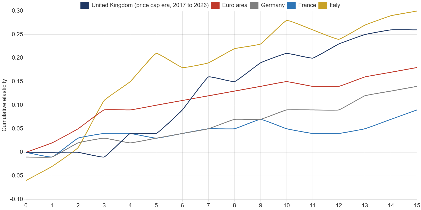
The results are clear. Britain does not have a low gas beta; it has one of the highest in Europe. After fifteen months, a 10 per cent rise in the wholesale gas price raises British household energy prices by about 2.6 per cent, against 1.8 per cent in the euro area, 1.4 per cent in Germany and 0.9 per cent in France. Only Italy, where gas-fired plants set the electricity price most of the time and retail tariffs follow wholesale prices closely, has a comparable exposure.
What is distinctive about Britain is the timing. In the euro area, about half of the long-run effect appears within three months. In Britain, under the price cap, nothing appears in the first three months, and half of the effect takes about seven months. The cap does not reduce exposure. It delays it, and then delivers it in large quarterly steps.
The electricity and gas components tell the same story. On the full sample, the fifteen-month elasticity is 0.30 for gas and 0.16 for electricity, reflecting the fact that gas sets the wholesale price of electricity only part of the time, and that network and policy costs make up a larger share of electricity bills.
2.3 Has the beta changed?
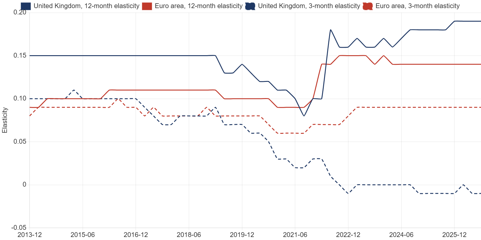
Figure 4 shows the 3-month and 12-month elasticities estimated over rolling eight-year windows. Two changes stand out. First, the British 3-month elasticity fell from about 0.10 before 2017 to zero after 2021: the introduction of the price cap removed the short-run pass-through entirely. Second, the British 12-month elasticity rose from about 0.11 in the windows ending in 2020 and 2021 to 0.19 in the windows ending in 2024 and 2025, above the euro area’s 0.14. The energy crisis of 2022 did not make Britain less sensitive to gas prices. It made it more sensitive, and more delayed.
This finding contradicts a widespread view that the growth of renewable generation has insulated British households from gas. Renewables have lowered the average cost of electricity, but as long as gas-fired plants set the marginal price for many hours of the year, wholesale electricity prices follow gas, and the price cap passes both through to households.
3. The Pipeline: Energy Inflation Already Locked In
Because the British pass-through is so delayed, a large part of the effect of gas prices already observed has not yet reached households. The estimated lag profile makes it possible to measure this pipeline directly: for each past change in the gas price, the model gives the share of its effect already passed through and the share still to come.
Table 3. Household energy price increases still in the pipeline from gas prices observed up to September 2026
| Horizon | Cumulative increase from September 2026 level | Implied index (2015 = 100) |
|---|---|---|
| December 2026 | 4 per cent | 193 |
| March 2027 | 11 per cent | 206 |
| June 2027 | 15 per cent | 213 |
| September 2027 | 18 per cent | 217 |
| December 2027 (full effect) | 19 per cent | 219 |
Note: assumes no further change in the wholesale gas price after September 2026. Starting index 184.6 in September 2026. Uncertainty: the standard error of the long-run elasticity implies a range of about 15 to 23 per cent for the full effect.
Table 3 shows the result. If the wholesale gas price stayed at its September 2026 level, British household energy prices would still rise by about 19 per cent, most of it in the first half of 2027. The steps coincide with the quarterly resets of the price cap in January and April. This is the part of the 2026 shock that Britain has not yet paid.
Translated into headline inflation, the pipeline is significant. A regression of the monthly change in the all-items index on the monthly change in the energy index gives an effective weight of 0.046. A 19 per cent increase in energy prices therefore adds about 0.9 points to the price level, spread over twelve months.
4. Monte Carlo Scenarios to 2028
The pipeline assumes that gas prices stay where they are. To account for uncertainty about future gas prices, the paper simulates 4,000 paths for the gas price from October 2026 to December 2028 under four assumptions. In the unconditional case, the gas price follows an autoregressive model estimated on 2010 to 2026 data, which pulls it slowly toward its long-run average of about 8.4 pounds, with shocks drawn in blocks of three months from the historical residuals. In three conditional scenarios, the price is pulled toward a target: 19 pounds if the shock persists, 10 pounds in a ceasefire, 30 pounds in an escalation. Each path is passed through the British distributed-lag model.
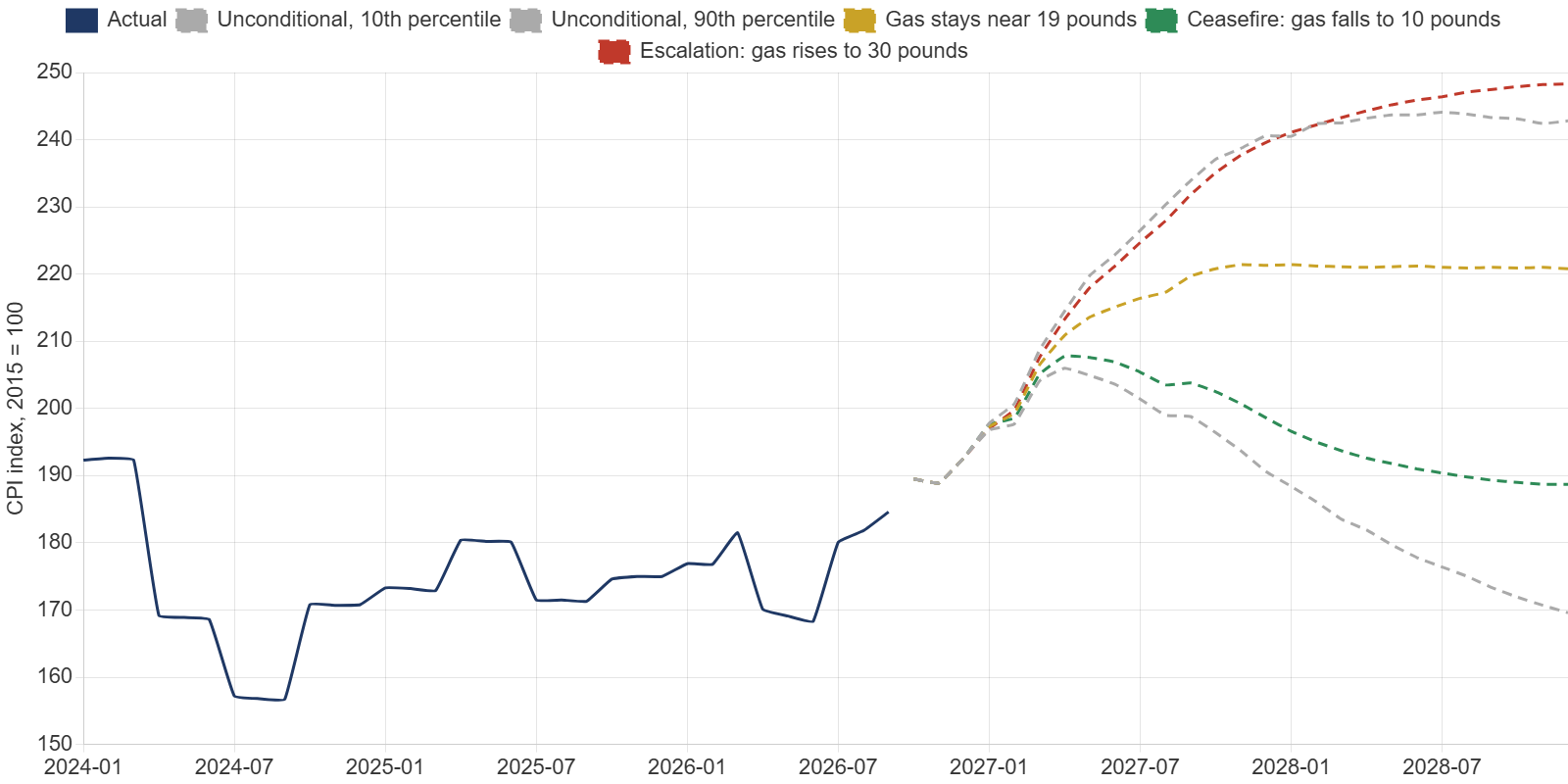
Table 4. Annual household energy inflation (%), median and 10th to 90th percentiles
| Scenario | January 2027 | April 2027 | July 2027 | December 2027 |
|---|---|---|---|---|
| Gas stays near 19 pounds | 11.5 (11.3 to 11.7) | 24.0 (22.0 to 26.0) | 20.2 (15.1 to 25.4) | 14.8 (7.4 to 23.6) |
| Ceasefire: gas falls to 10 pounds | 11.7 (11.4 to 11.9) | 22.1 (20.3 to 23.8) | 14.0 (9.9 to 18.2) | 3.1 (-2.4 to 9.4) |
| Escalation: gas rises to 30 pounds | 11.4 (11.1 to 11.6) | 25.4 (23.3 to 27.5) | 24.8 (20.2 to 30.2) | 24.3 (17.6 to 32.3) |
| Unconditional | 11.5 (11.2 to 11.8) | 23.6 (21.1 to 26.1) | 18.5 (11.8 to 25.8) | 10.7 (-1.1 to 24.9) |
Note: annual change in CPI index 04.5. September 2026: 7.8 per cent.
The striking result is how little the scenarios differ in the first half of 2027. In April 2027, annual household energy inflation is between 22 and 25 per cent in every scenario, and the probability that it exceeds 20 per cent is 92 per cent even in the ceasefire scenario. The January and April 2027 increases are already determined by gas prices observed in 2026. The scenarios only diverge from the summer of 2027: by December 2027, energy inflation ranges from 3 per cent in a ceasefire to 24 per cent in an escalation.
Table 5. Contribution of household energy to annual CPI inflation (percentage points)
| Scenario | September 2026 (actual) | April 2027 | December 2027 |
|---|---|---|---|
| Gas stays near 19 pounds | 0.36 | 1.10 | 0.68 |
| Ceasefire | 0.36 | 1.02 | 0.14 |
| Escalation | 0.36 | 1.17 | 1.12 |
Note: annual energy inflation times the estimated effective weight of 0.046.
For monetary policy, this has an uncomfortable implication. The energy contribution to headline inflation will roughly triple between September 2026 and April 2027, adding about 0.7 points to headline inflation, even if a ceasefire brings gas prices down. A central bank that reacts to the April 2027 inflation figure will be reacting to gas prices of mid-2026. The first paper in this series argued that the November 2026 hike responded to a supply shock; the pipeline identified here suggests that headline inflation will rise again in early 2027 regardless of what the Bank does.
5. The Industrial Side: Scars That Do Not Heal
Households are not the only channel of exposure. Energy-intensive industries, chemicals, basic metals, glass, cement and ceramics, and paper, use gas as fuel and feedstock and compete with producers in regions where energy is cheaper. Figure 6 shows their output since 2015.
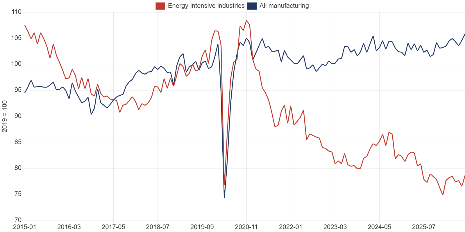
The decline is severe. Chemicals output in August 2026 was 42 per cent below its January 2021 level and non-metallic minerals output 36 per cent lower, while total manufacturing output was 5 per cent higher. The energy-intensive index has fallen by about 30 per cent relative to manufacturing since 2021. Most of the damage was done in 2022 and 2023, and it was not reversed when gas prices fell back in 2024.
To measure the industrial gas beta, the paper estimates local projections of energy-intensive output on the three-month change in the gas price, separating increases from decreases, with controls for past output growth and past gas price changes, on monthly data from 1998 to August 2026.
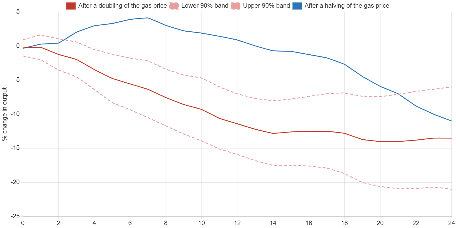
Table 6. Response of energy-intensive output to the gas price
| Shock | After 6 months | After 12 months | After 24 months |
|---|---|---|---|
| Doubling of the gas price | -5.5% | -11.4% (se 2.7) | -13.5% (se 4.6) |
| Halving of the gas price | not significant | +0.9% | -11.0% |
| Memo: all gas changes, per doubling | -3.8% | -5.3% | -1.5% |
Note: local projections, HAC standard errors. The symmetric estimate is shown for comparison.
The results reveal a strong asymmetry. A doubling of the gas price reduces energy-intensive output by about 11 per cent after one year and 13.5 per cent after two, and the effect is statistically significant. A halving of the gas price does not raise output at all; if anything, output keeps falling, because falls in gas prices often coincide with recessions. Plants that close when gas is expensive do not reopen when it becomes cheaper. A symmetric model, which averages the two, badly understates the damage from price spikes.
Applied to 2026, the asymmetric estimates imply that the 76 log-point rise in the sterling gas price since January would reduce energy-intensive output by about 10 to 15 per cent by 2028, from a base already 30 per cent smaller than in 2021. So far the effect is not visible: energy-intensive output in August 2026 was slightly higher than in February. The lag structure suggests the losses will show up in 2027. For the economy as a whole, by contrast, the estimated response of monthly GDP to gas prices is small and not statistically significant: the industries most exposed now account for a small share of output.
6. Implications for Policy
Three conclusions follow for policy makers.
For the Bank of England, the main implication is that a second wave of energy inflation is coming in the first half of 2027 and is largely independent of future gas prices. A central bank that has already tightened against the 2026 shock should treat that wave as the delayed arrival of a known shock, not as new information about inflation pressure. Communicating this now would reduce the risk that the April 2027 inflation figure triggers a further, unnecessary tightening.
For the government, the price cap creates a window of decision. The April 2027 cap will be set from wholesale prices observed over the winter, and its level can be anticipated with reasonable precision. Any support for households, whether through bill rebates or temporary changes to policy costs in bills, can be prepared in advance and targeted. The timing advantage that the cap gives Britain is only useful if it is used.
For industrial policy, the asymmetry of the industrial gas beta matters most. Energy-intensive industries lose capacity when gas prices spike and do not regain it when prices fall. Support that arrives after the spike, or that is designed only to cover price peaks, will not prevent permanent closures. Mechanisms that cap the input cost of gas for exposed industries during spikes, or that accelerate their access to cheaper electricity, are more likely to preserve capacity than compensation after the fact.
7. Conclusions
Britain’s apparent resilience to the 2026 gas shock is an illusion of timing. The British gas beta is among the highest in Europe; it is simply delivered later and in larger steps. About 19 per cent of further household energy price increases are already locked in by gas prices observed in 2026, and they will arrive in January and April 2027 whatever happens next. On the industrial side, each spike leaves a lasting mark on an already diminished energy-intensive sector. Measuring the gas beta, and its timing, is therefore essential to anticipating Britain’s inflation and output in 2027.
Methodological Appendix
A1. Distributed-lag model
For each country, the equation is dp(t) = sum over l from 0 to 15 of b(l) dg(t-l) + monthly dummies + e(t), where dp is the monthly log change of household energy prices times 100 and dg the monthly log change of the wholesale gas price times 100. Estimated by least squares with Newey-West standard errors (12 lags). The cumulative elasticity at lag k is the sum of b(0) to b(k); its standard error uses the full covariance matrix. For the British price-cap model, b(0) to b(2) are set to zero; the unrestricted estimates are reported in Table 2 for the full sample.
A2. Pipeline and Monte Carlo
The pipeline at horizon h is the sum over past gas changes dg(T-l), l from 0 to 15, of dg(T-l) times [C(min(l+h, 15)) – C(l)], where C is the cumulative elasticity and T is September 2026. In the Monte Carlo, the log gas price follows x(t) = x(t-1) + k [target – x(t-1)] + u(t), with k = 0.16 (0.10 in the persistence scenario) and u drawn in blocks of three months from the residuals of an AR(1) model estimated on 2010 to 2026 data and scaled by 0.8. In the unconditional case, x follows the estimated AR(1) itself (autoregressive coefficient 0.973, long-run mean 8.4 pounds). Energy prices are then computed by applying the distributed-lag coefficients to the simulated gas changes.
A3. Local projections
For horizons h from 0 to 24, y(t+h) – y(t-1) is regressed on the positive and negative parts of the three-month log change in the gas price, two lags of output growth and the lagged three-month gas change, with Newey-West standard errors (h+1 lags). y is 100 times the log of the energy-intensive index. Coefficients are scaled to a doubling (69.3 log points) or halving of the gas price.
A4. Limitations
The models are reduced-form and assume that the relation between wholesale and retail prices is stable within each sample. Changes to the methodology of the price cap, government support schemes such as the 2022 Energy Price Guarantee, and changes in hedging behaviour by suppliers all affect the pass-through and are only partly captured. The TTF benchmark is used for Britain because the NBP price is not available on FRED; the two are highly correlated but not identical. The industrial estimates do not separate gas from electricity costs, and cannot distinguish closures from temporary cuts in production.
References
Eurostat (2026), Harmonised indices of consumer prices, accessed via FRED, November 2026.
Ofgem (2026), Energy price cap methodology.
Office for National Statistics (2026), Consumer price inflation, September 2026; Index of production, August 2026.
World Bank (2026), Commodity price data (Pink Sheet), accessed via FRED, November 2026.
Driss EFFINA, PhD
Independent Researcher, Global Strategy Files
The opening pages of our four country reports: United States, United Kingdom, Japan and China. A free PDF, sent to your inbox.
You will also receive occasional analysis from Global Strategy Files. Unsubscribe in one click, at any time.