The Supply-Shock Trap: Why the Bank of England Is Tightening into a Weak Economy

Download PDF
Executive Summary
On 5 November 2026 the Bank of England raised Bank Rate by a quarter point to 4 per cent, its first increase since August 2023, and warned that at least one more increase was likely if the conflict between the United States and Iran continued. The Bank expects consumer price inflation, 3.5 per cent in September, to approach 5 per cent by the middle of 2027, driven by oil and gas prices. The economy it is tightening into is weak: unemployment is close to 5 per cent, the Office for Budget Responsibility has cut its growth forecast for 2027 to 1 per cent, and mortgage rates on new fixed deals have reached a three-year high.
The question the Monetary Policy Committee faces is not whether inflation will rise. It will. The question is how much of the energy shock will feed into domestic prices and wages, the so-called second-round effects that monetary policy can influence, as opposed to the first-round rise in energy bills that it cannot. This paper answers that question with the latest official data and four complementary methods. Five findings stand out.
- Second-round effects depend on the labour market, and today’s labour market is loose. Local projections estimated on monthly data since 2001 show that the response of core inflation to an energy price shock rises steeply with the ratio of vacancies to unemployed people. At the 2022 ratio of 1.04, a 10 per cent rise in energy prices added about 0.30 percentage points to core inflation a year later. At the 2026 ratio of 0.42, the same shock adds about 0.09 points. For services inflation the gap is wider still: 0.45 points against 0.05.
- Applied to the actual 2026 shock, energy prices up 69 per cent on a year earlier in September, the models imply a peak addition of about 0.6 points to core inflation and 0.35 points to services inflation. The same shock in the labour market of 2022 would have added about 2.1 and 3.1 points respectively.
- A structural VAR identified with sign restrictions attributes almost all of the 2026 inflation overshoot to supply shocks, with demand shocks contributing slightly negatively. In October 2022, by contrast, demand and loose monetary conditions together accounted for about 2.8 points of inflation, against 3.1 points for supply. The 2022 episode was half a demand problem; 2026 is a supply problem.
- Wage indexation, the pass-through of past inflation into pay, peaked at 0.44 in the five years to 2023 and has fallen to 0.20. Even if inflation reached 5 per cent, the estimated wage equation implies regular pay growth of about 4.4 per cent, compared with 7.8 per cent in mid-2023. Long-term inflation expectations in the gilt market have not moved: the five-year, five-year forward rate is lower than in 2022 and does not respond to inflation news.
- A 25 basis point tightening lowers the price level by about 0.7 per cent after two years in the central estimate, with a wide band from 0.3 to 1.5 per cent, and lowers GDP by about 0.5 per cent. A second hike would therefore remove roughly as much inflation as the entire second-round effect the data predict, at a cost of around 16 billion pounds of output.
The first hike is defensible. A simple policy rule based on core inflation and the unemployment gap prescribed exactly 4 per cent in September 2026, and a central bank that has just lived through 2022 has good reasons to buy insurance. But the evidence points to a narrow margin between insurance and overkill. The Bank of England risks fighting the last war: tightening against a wage-price spiral that the current labour market is unlikely to generate, at the cost of real output in an economy already close to stagnation.
1. The November Dilemma
The Bank of England’s decision of 5 November 2026 was its first rate rise since the end of the 2021 to 2023 tightening cycle. It was widely expected, voted 8 to 1 with no member in favour of holding, and accompanied by a message that more increases were likely if the conflict in the Middle East persisted. The case for the hike is easy to state. Headline inflation rose from 2.6 per cent in June to 3.5 per cent in September 2026. Core inflation, which excludes energy, food, alcohol and tobacco, edged up from 2.6 to 2.8 per cent. Services inflation reached 3.7 per cent. Brent crude in sterling terms was more than 60 per cent higher than a year earlier, and European gas prices had more than doubled since the spring.
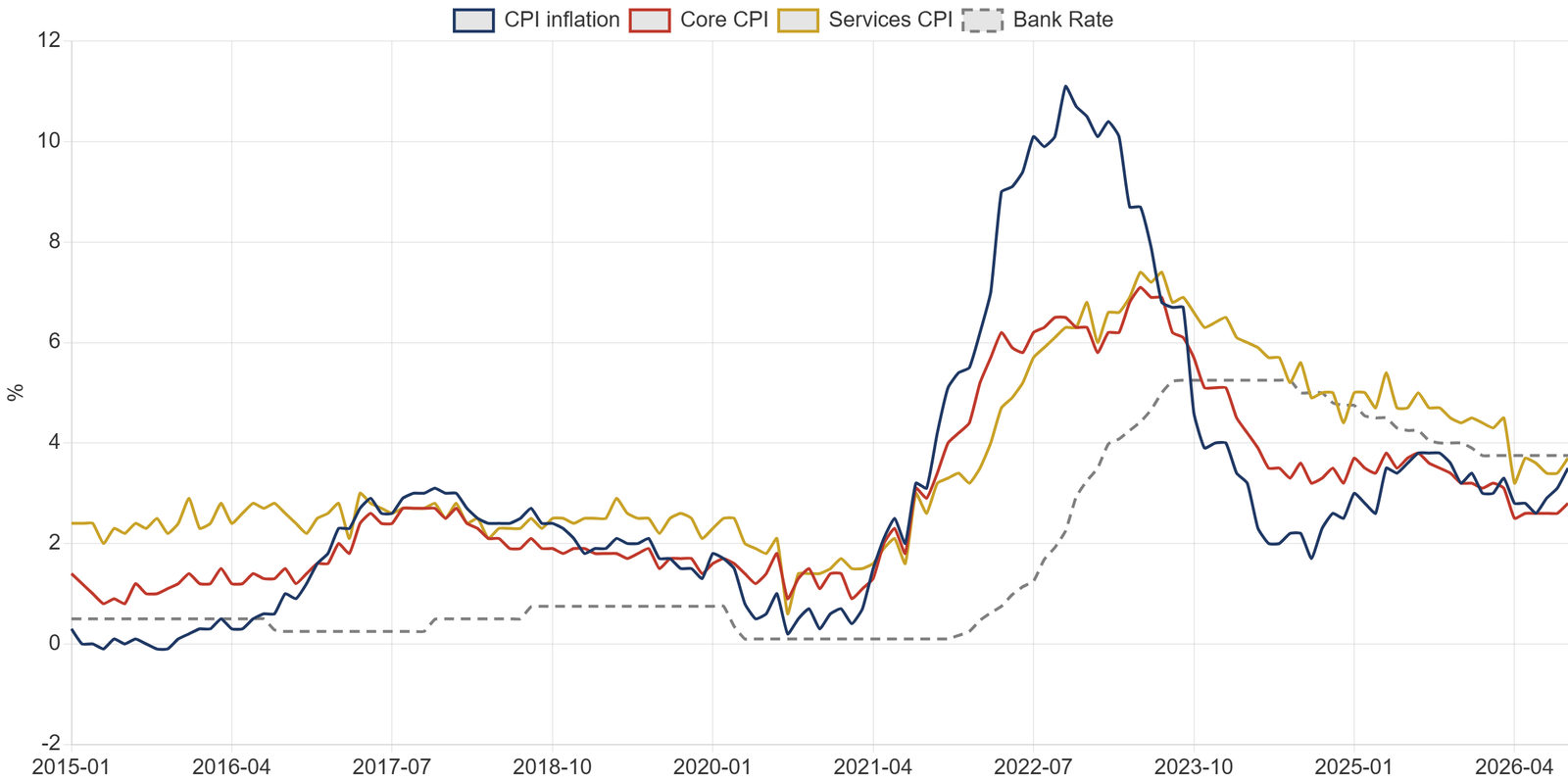
The case against the hike is just as easy to state. The shock is imported. It reduces real incomes and demand on its own, as households pay more for energy and less for everything else. The labour market has been loosening for three years: unemployment rose from 3.6 per cent in mid-2022 to around 4.7 to 5.1 per cent in 2026, and vacancies have fallen from 1.3 million to under 700,000. Pay growth has slowed to below 4 per cent. If the energy shock does not feed into domestic wages and services prices, monetary tightening will add a demand contraction to a supply contraction without changing the medium-term inflation outlook.
Between these two cases lies an empirical question, and it is the one this paper addresses: how large are the second-round effects of the 2026 energy shock likely to be, given the state of the British economy today? The question cannot be answered by analogy with 2022, because the economy of 2026 is different in at least three respects: the labour market is far looser, inflation expectations are more firmly anchored, and the monetary stance before the shock was already restrictive rather than at emergency settings.

Figure 2 compares the two shocks. Measured in sterling, the 2022 shock was larger: a composite of European gas and Brent crude prices rose by up to 130 per cent over twelve months in 2022, against 69 per cent in the year to September 2026. Oil now plays a larger role and gas a smaller one, which matters because gas sets the price of British electricity at the margin and was the main channel through which the 2022 shock reached household bills. The 2026 shock is serious, and the Ofgem price cap has risen by 13.5 per cent in July and a further 4 per cent in October, but it is not a repeat of 2022.
1.1 Data and methods
The analysis uses monthly official data from 1997 to September or October 2026 (Table 1). Four methods are combined. State-dependent local projections estimate how the response of core and services inflation to energy price shocks varies with labour market tightness. A sign-restricted structural vector autoregression separates supply, demand and monetary shocks and decomposes inflation into their contributions. A wage equation measures the indexation of pay to past inflation and how it has changed. Finally, the paper measures the anchoring of market-based inflation expectations and the effect of a monetary tightening on output and prices.
Table 1. Data used in this paper
| Series | Source | Span |
|---|---|---|
| CPI, core CPI, services CPI, CPI index | Office for National Statistics (MM23) | Monthly, 1989 to Sep 2026 |
| Unemployment rate, vacancies | Office for National Statistics (LMS) | Monthly, 1971 and 2001 to Aug 2026 |
| Average weekly earnings, regular pay level and growth | Office for National Statistics (LMS) | Monthly, 2000 to Aug 2026 |
| Monthly gross value added | Office for National Statistics | Monthly, 1997 to Aug 2026 |
| Bank Rate, sterling exchange rates | Bank of England | Monthly, 1990 to Oct 2026 |
| Nominal and implied inflation zero-coupon curves | Bank of England | Monthly, 1979 to Oct 2026 |
| Brent crude and European natural gas prices | FRED (US EIA and IMF data) | Monthly, 1995 to Oct 2026 |
Note: the unemployment rate refers to the rolling three-month period centred on the month shown.
2. Anatomy of the Shock: Energy, Labour and Expectations
Second-round effects arise through three channels. Firms pass higher energy costs into the prices of other goods and services. Workers seek compensation for lost purchasing power in higher wages, which firms pass on in turn. And if households and firms come to expect higher inflation, they build it into price and wage setting regardless of costs. The strength of each channel depends on the state of the economy.
On the first channel, the 2026 shock arrives in an economy where firms have less pricing power than in 2022. Demand is weak, retail and hospitality insolvencies remain historically high, and the post-pandemic reopening that allowed firms to widen margins in 2021 and 2022 has no equivalent today. On the second channel, the labour market is the decisive difference (Figure 3). In June 2022 there were 1.04 vacancies for every unemployed person, the tightest ratio on record; in mid-2026 the ratio was 0.42, below its pre-pandemic level of 0.60. Regular pay growth, which peaked at 7.8 per cent in the three months to August 2023, was 3.7 per cent in August 2026, and private sector pay growth was 3.0 per cent.

On the third channel, the evidence from financial markets is reassuring (Figure 8). Five-year implied RPI inflation from the index-linked gilt market rose from 3.1 per cent in mid-2025 to 3.7 per cent in September 2026, reflecting the near-term energy shock. But the five-year rate starting five years ahead, which measures the credibility of the inflation target, was 3.0 to 3.1 per cent, lower than in 2022 and close to its long-run average once the usual wedge of around 0.8 to 1 point between RPI and CPI inflation is taken into account. Markets expect the shock to pass.
3. How Much Will Energy Feed Into Domestic Inflation?
3.1 A state-dependent model of pass-through
To measure second-round effects, the paper estimates local projections in the spirit of Jordà (2005). For each horizon h from 0 to 24 months, the change in core (or services) inflation between month t-1 and month t+h is regressed on the twelve-month percentage change in a composite energy price index in sterling, built from European natural gas and Brent crude with equal weights; on the interaction of that energy shock with the ratio of vacancies to unemployed people, measured relative to its pre-pandemic level; on the labour market ratio itself; on lagged inflation; and on the change in Bank Rate. Standard errors are corrected for the overlapping horizons. The sample runs from June 2001 to September 2026.
The interaction term is the heart of the exercise. It allows the pass-through of energy into core and services prices to differ according to how tight the labour market is when the shock hits. Table 2 reports the two key coefficients.
Table 2. Pass-through of energy prices to core and services inflation: local projection estimates
| Horizon (months) | Core: energy shock | Core: energy x tightness | Services: energy shock | Services: energy x tightness |
|---|---|---|---|---|
| 0 | 0.0017 (3.8) | 0.0053 (2.7) | 0.0017 (4.3) | 0.0041 (2.3) |
| 6 | 0.0104 (3.6) | 0.0232 (2.2) | 0.0102 (6.1) | 0.0311 (4.1) |
| 12 | 0.0155 (3.3) | 0.0335 (3.2) | 0.0157 (4.7) | 0.0590 (4.9) |
| 18 | 0.0118 (2.0) | 0.0378 (2.3) | 0.0152 (3.2) | 0.0662 (4.0) |
| 24 | 0.0056 (0.8) | 0.0233 (1.1) | 0.0118 (2.5) | 0.0501 (2.7) |
Note: coefficients on the twelve-month percentage change in the sterling energy composite and on its interaction with the vacancy-to-unemployment ratio (minus 0.6). HAC t-statistics in parentheses. Dependent variable: change in the annual inflation rate between t-1 and t+h, percentage points. Monthly data, June 2001 to September 2026.
The interaction coefficients are positive, large and statistically significant at every horizon up to 18 months. Energy shocks feed into core and services inflation far more when the labour market is tight. Figures 4 and 5 translate the estimates into the response to a 10 per cent rise in energy prices under the labour market conditions of June 2022 and of mid-2026.


The difference is striking. In the 2022 labour market, a 10 per cent energy shock raised core inflation by about 0.30 points after a year, and services inflation by about 0.45 points after 15 months. In the 2026 labour market, the same shock raises core inflation by about 0.09 points and services inflation by about 0.05 points. The pass-through into core inflation is roughly three times weaker; the pass-through into services, the component most closely watched by the Monetary Policy Committee because it reflects domestic labour costs, is about nine times weaker.
3.2 What the 2026 shock implies
Table 3. Implied second-round effects of the 2026 energy shock (percentage points)
| Measure | 2026 shock, 2026 labour market | 2026 shock, 2022 labour market | 2022 shock, 2022 labour market |
|---|---|---|---|
| Energy composite, 12-month change (%) | +69 | +69 | +130 |
| Core inflation, peak effect | +0.6 | +2.1 | +3.9 |
| Services inflation, peak effect | +0.35 | +3.1 | +5.9 |
| Months to peak (core, services) | 9 to 12 | 12 to 15 | 12 to 15 |
Note: peak effects computed as the energy shock multiplied by the state-dependent coefficient at the peak horizon. The 2022 shock uses the maximum twelve-month change in the composite during 2021 and 2022.
Table 3 applies the estimates to the actual shocks. The 69 per cent rise in the energy composite in the year to September 2026 implies a peak addition of about 0.6 points to core inflation and 0.35 points to services inflation, spread over the coming year. Had the same shock struck the labour market of 2022, the additions would have been about 2.1 and 3.1 points. The 2022 shock itself, twice as large and hitting a tight labour market, implies effects of about 4 and 6 points, which is close to what actually happened: core inflation rose from about 1 per cent in early 2021 to 7.1 per cent in May 2023, and services inflation to 7.4 per cent.
The implication for policy is direct. The second-round component of the 2026 shock, the part that monetary policy exists to prevent, is likely to be modest: about half a point of core inflation at its peak. The first-round effect on headline inflation will be much larger, and the Bank’s projection of inflation close to 5 per cent by mid-2027 is plausible. But most of that rise will reverse when energy prices stabilise, whatever the Bank does.
4. Supply or Demand? A Structural Decomposition
The local projections isolate one channel. A complementary approach asks a broader question: how much of British inflation in each period has been driven by supply shocks, which push prices up and output down, by demand shocks, which push both up, and by monetary shocks? The paper estimates a vector autoregression with monthly growth in gross value added, seasonally adjusted monthly CPI inflation and the 2-year gilt yield as the measure of the policy stance, with the energy price composite as an exogenous variable, from 1998 to August 2026. Shocks are identified with sign restrictions in the tradition of Uhlig (2005) and Rubio-Ramirez, Waggoner and Zha (2010): a supply shock lowers output and raises prices; a demand shock raises output, prices and interest rates; a monetary shock raises interest rates and lowers output and prices. The restrictions hold for three months. Of 40,000 random rotations, 11,543 satisfy them, and the results are reported for the rotation closest to the median responses.

Table 4. Contributions of structural shocks to twelve-month inflation (percentage points)
| Month | Supply shocks | Demand shocks | Monetary shocks |
|---|---|---|---|
| December 2021 | +0.87 | -0.05 | -0.14 |
| October 2022 | +3.07 | +1.64 | +1.15 |
| June 2023 | +1.85 | +3.00 | +0.29 |
| June 2024 | -0.27 | +0.39 | -0.21 |
| June 2025 | +0.64 | +0.29 | +0.43 |
| March 2026 | +0.55 | +0.16 | +0.34 |
| August 2026 | +0.52 | -0.13 | -0.04 |
Note: historical decomposition from the sign-restricted VAR. Contributions are relative to the deterministic baseline and exclude the direct effect of the exogenous energy price variable.
Table 4 and Figure 6 tell a clear story. At the peak of the 2022 episode, in October 2022, supply shocks contributed about 3.1 points to inflation, but demand shocks and loose monetary conditions together contributed another 2.8 points. By June 2023, as energy prices fell, the demand component had become the largest single source of inflation, at 3 points: the legacy of a tight labour market, fiscal support and a slow monetary response. The 2022 to 2023 inflation was, in roughly equal measure, a supply shock and a demand problem.
The 2026 picture is different. In August 2026, before the full effect of the war on energy prices, supply shocks contributed about half a point, while demand and monetary shocks contributed slightly negatively. There is no evidence of excess demand pressure in the British economy. The inflation the Bank is now confronting comes almost entirely from the supply side.
5. Wages and Expectations: The Missing Spiral
5.1 Wage indexation
The channel that turned the 2022 energy shock into persistent inflation was pay. Workers who had lost purchasing power demanded compensation, and in a tight labour market they obtained it. To measure how strongly pay responds to past inflation, the paper estimates a simple wage equation on monthly data from 2002 to 2026: regular pay growth regressed on the unemployment rate, CPI inflation three months earlier and five-year market inflation expectations.
Table 5. Wage equation: regular pay growth, 2002 to 2026
| Variable | Coefficient | t-statistic |
|---|---|---|
| Constant | 5.36 | 4.1 |
| Unemployment rate (%) | -0.66 | 5.3 |
| CPI inflation, three months earlier (%) | 0.32 | 4.7 |
| Five-year implied inflation (%) | 0.23 | 0.8 |
| R-squared | 0.57 |
Note: dependent variable is the growth of regular average weekly earnings, three-month average on a year earlier. HAC standard errors with 12 lags.
Over the whole period, each point of past inflation adds about a third of a point to pay growth, and each point of unemployment subtracts two thirds of a point. But the indexation coefficient is not stable (Figure 7). Estimated over rolling five-year windows, it was close to zero or negative through the 2010s, when inflation was low and workers had little bargaining power, jumped to about 0.44 in the window ending in 2023, and has since fallen back to about 0.20.

Using the full-sample equation, inflation of 5 per cent in 2027 combined with unemployment of 5.2 per cent would imply regular pay growth of about 4.4 per cent, against 3.9 per cent if inflation stayed at 3.5 per cent. With productivity growth of around 1 per cent, pay growth of 4.4 per cent is consistent with unit labour cost growth of about 3.4 per cent, uncomfortable for a few quarters but far from the 7 to 8 per cent pay growth of 2023. Using the more recent rolling coefficient of 0.2, the pass-through would be smaller still.
5.2 Expectations

The final channel is expectations. If the energy shock persuaded households and firms that the Bank would tolerate higher inflation, the second-round effects would be larger than any backward-looking model suggests. The gilt market provides a continuous test. Table 6 reports the sensitivity of monthly changes in five-year and five-year forward implied inflation to monthly changes in CPI inflation in three periods.
Table 6. Do market inflation expectations respond to inflation news?
| Period | Five-year implied inflation | Five-year, five years forward |
|---|---|---|
| 2010 to 2019 | 0.068 (1.3) | 0.028 (0.5) |
| 2021 to 2023 | 0.030 (0.7) | -0.029 (0.9) |
| 2024 to Sep 2026 | -0.001 (0.0) | -0.013 (0.4) |
Note: coefficient on the monthly change in CPI inflation; robust t-statistics in parentheses.
In none of the three periods do long-term expectations react significantly to inflation news, and the five-year, five-year forward rate in October 2026, at 3.04 per cent in RPI terms, was below its level of 3.56 per cent in June 2022. Expectations were not the problem in 2022, and they are not the problem now. This does not make them irrelevant: anchored expectations are partly the product of the Bank’s demonstrated willingness to act. But it does mean that the credibility case for a second hike is weaker than the credibility case for the first.
6. Policy Rules, Costs and Counterfactuals
6.1 What a simple rule prescribes
A useful benchmark is the policy rule proposed by Taylor (1993), in which the policy rate equals a neutral real rate plus inflation, plus half the gap between inflation and the target, plus half the output gap. The paper computes two versions, one using core inflation and one using headline inflation, with a neutral real rate of 1 per cent and an output gap derived from the unemployment gap relative to an equilibrium rate of 4.5 per cent, using an Okun coefficient of 2.

The comparison is instructive. In 2022 Bank Rate stood 6 to 8 points below the core-based rule, the clearest sign that policy was behind the curve. In September 2026 the core-based rule prescribed 4.0 per cent, exactly the rate chosen in November; the headline-based rule prescribed about 5 per cent. The choice between the two rules is the choice the Committee faces. Responding to headline inflation means responding to the first-round effect of energy prices, which a central bank normally looks through. Responding to core inflation means responding to what remains once energy and food are excluded. On the core measure, the November hike is justified; a second hike would require core inflation to rise by about another half point, which is roughly the second-round effect estimated in Section 3.
6.2 The cost of tightening
The same structural VAR delivers an estimate of the effect of a monetary tightening. Figure 10 shows the response of output and prices to a shock that raises the 2-year gilt yield by 25 basis points on impact.

Table 7. The arithmetic of a second hike
| Item | Central estimate | Cautious estimate |
|---|---|---|
| Price level effect of 25 bp after 24 months | -0.68% | -0.34% |
| GDP effect of 25 bp after 24 months | -0.53% | -0.10% |
| Second-round effect on core inflation to be offset (Section 3) | +0.6 pp | +0.6 pp |
| GDP cost of a second hike (2026 prices) | about 16.7 billion pounds | about 3 billion pounds |
| Output cost per point of inflation removed (sacrifice ratio) | 0.8 | 0.3 |
Note: central estimate is the median response; cautious estimate uses the 84th percentile of the price response and the corresponding GDP response bound. Nominal GDP of 3.15 trillion pounds. Ranges are wide and should be read as orders of magnitude.
In the central estimate, a 25 basis point tightening lowers the price level by about 0.7 per cent after two years and GDP by about 0.5 per cent. The band is wide, as it always is for monetary policy effects, from 0.3 to 1.5 per cent for prices. Even so, the arithmetic is sobering. A second quarter-point increase would remove roughly as much inflation over two years as the entire second-round effect of the energy shock that the local projections predict, and it would do so at a central cost of around 16 billion pounds of output. The Bank would be using a demand instrument to offset a supply-driven rise in prices that is likely to reverse on its own, in an economy where demand is already falling.
7. Conclusions and Scenarios for 2027
The November 2026 hike was the right kind of mistake to risk. A central bank that had misread the 2021 to 2022 inflation shock as transitory could not afford to be seen to hesitate again, and a simple core-based rule supported the move. But the evidence assembled in this paper suggests that the macroeconomic case for going further is weak. The labour market is loose, and the state-dependent estimates imply second-round effects about three times weaker for core inflation and up to nine times weaker for services than in 2022. The structural decomposition finds no demand-driven inflation in 2026. Wage indexation has halved. Long-term expectations are anchored.
Table 8. Three scenarios for 2027
| Scenario | Energy prices | Core inflation, mid-2027 | Policy implication |
|---|---|---|---|
| A. War persists, prices plateau | Composite stays near Q4 2026 level | 3.2 to 3.5% | Hold at 4.0%; headline inflation falls back from late 2027 |
| B. Escalation, Hormuz closed for longer | Further 30 to 50% rise | 3.6 to 4.0% | Case for a second hike if services inflation and pay accelerate together |
| C. Ceasefire | Composite falls 30% | 2.4 to 2.8% | Reverse the November hike within two to three meetings |
Note: indicative ranges combining the pass-through estimates of Section 3 with core inflation of 2.8 per cent in September 2026.
The paper’s central conclusion is that the Bank should set a higher bar for the second hike than for the first. The relevant test is not the headline rate, which will rise mechanically with energy prices, but evidence that the shock is spreading through services prices and pay at the same time. On the evidence available in November 2026, that test is not met, and the models suggest it is unlikely to be met unless the shock grows much larger. The risk of the coming year is not a wage-price spiral. It is a central bank that, having been too slow in 2022, is now too quick, and turns an imported energy shock into a domestic recession.
Methodological Appendix
A1. Local projections
For horizons h = 0, 3, 6 and so on up to 24, the equation is pi(t+h) – pi(t-1) = a + b E(t) + c E(t) x (VU(t) – 0.6) + d (VU(t) – 0.6) + f (pi(t-1) – pi(t-13)) + g dR(t) + u(t+h), where pi is core or services inflation, E is the twelve-month percentage change in the energy composite (0.5 log gas price plus 0.5 log Brent price, in sterling), VU is vacancies divided by the number of unemployed people and dR is the twelve-month change in Bank Rate. The state-dependent response at tightness VU* is b + c (VU* – 0.6). Standard errors are Newey-West with h+1 lags.
A2. Structural VAR
The reduced-form VAR has six lags of monthly GVA growth, seasonally adjusted monthly CPI inflation (monthly means removed, 1998 to 2019) and the 2-year zero-coupon gilt yield, with current and three lags of the monthly change in the energy composite as exogenous regressors, January 1998 to August 2026. Structural impact matrices are drawn as the Cholesky factor of the residual covariance times random orthogonal matrices (QR decomposition of Gaussian draws). Sign restrictions are imposed on cumulative output and price responses and on the yield response for months 0 to 2. The reported rotation minimises the standardised distance to the median responses (Fry and Pagan, 2011). The historical decomposition sums the contributions of each identified shock to monthly inflation over twelve months.
A3. Wage equation and rules
The wage equation uses the growth of regular average weekly earnings (three-month average on a year earlier) computed from the ONS level series. Rolling coefficients use 60-month windows with unemployment and lagged inflation only. The Taylor rule is i = 1 + pi + 0.5 (pi – 2) + 0.5 y, with y = -2 (u – 4.5).
A4. Limitations
The energy composite is a proxy for the cost shock faced by British firms and households; regulated retail energy prices respond with a lag through the Ofgem price cap. The vacancy-to-unemployment ratio summarises labour market tightness imperfectly, and the interaction model assumes a linear dependence of pass-through on tightness. Sign-restricted VARs identify sets of models rather than unique ones, and the monetary policy effects in particular carry wide uncertainty. The scenario ranges in Table 8 are indicative.
References
Bank of England (2026), Monetary Policy Report, November 2026.
Fry, R. and Pagan, A. (2011), Sign restrictions in structural vector autoregressions: a critical review, Journal of Economic Literature, 49(4), 938-960.
Jordà, O. (2005), Estimation and inference of impulse responses by local projections, American Economic Review, 95(1), 161-182.
Office for Budget Responsibility (2026), Economic and fiscal outlook, October 2026.
Office for National Statistics (2026), Consumer price inflation, September 2026; Labour market overview, October 2026.
Ofgem (2026), Energy price cap decisions for July to September and October to December 2026.
Rubio-Ramirez, J. F., Waggoner, D. F. and Zha, T. (2010), Structural vector autoregressions: theory of identification and algorithms for inference, Review of Economic Studies, 77(2), 665-696.
Taylor, J. B. (1993), Discretion versus policy rules in practice, Carnegie-Rochester Conference Series on Public Policy, 39, 195-214.
Uhlig, H. (2005), What are the effects of monetary policy on output? Results from an agnostic identification procedure, Journal of Monetary Economics, 52(2), 381-419.
Driss EFFINA, PhD
Independent Researcher, Global Strategy Files
The opening pages of our four country reports: United States, United Kingdom, Japan and China. A free PDF, sent to your inbox.
You will also receive occasional analysis from Global Strategy Files. Unsubscribe in one click, at any time.